Table of contents
- About DisplayCAL
- Disclaimer
- Download
- Quickstart guide
- System requirements and other prerequisites
- Installation
- Basic concept of display calibration
- A note about colorimeters, displays and DisplayCAL
- Usage
- Menu commands
- Scripting
- User data and configuration file locations
- Known issues & solutions
- Get help
- Report a bug
- Discussion
- To-Do / planned features
- Thanks and acknowledgements
- Version history / changelog
- Definitions
About DisplayCAL
DisplayCAL (formerly known as dispcalGUI) is a display calibration and profiling solution with a focus on accuracy and versatility (in fact, the author is of the honest opinion it may be the most accurate and versatile ICC compatible display profiling solution available anywhere). At its core it relies on ArgyllCMS, an advanced open source color management system, to take measurements, create calibrations and profiles, and for a variety of other advanced color related tasks.
Calibrate and characterize your display devices using one of many supported measurement instruments, with support for multi-display setups and a variety of available options for advanced users, such as verification and reporting functionality to evaluate ICC profiles and display devices, creating video 3D LUTs, as well as optional CIECAM02 gamut mapping to take into account varying viewing conditions. Other features include:
- Support of colorimeter corrections for different display device types to increase the absolute accuracy of colorimeters. Corrections can be imported from vendor software or created from measurements if a spectrometer is available.
- Check display device uniformity via measurements.
- Test chart editor: Create charts with any amount and composition of color patches, easy copy & paste from CGATS, CSV files (only tab-delimited) and spreadsheet applications, for profile verification and evaluation.
- Create synthetic ICC profiles with custom primaries, white- and blackpoint as well as tone response for use as working spaces or source profiles in device linking (3D LUT) transforms.
Screenshots
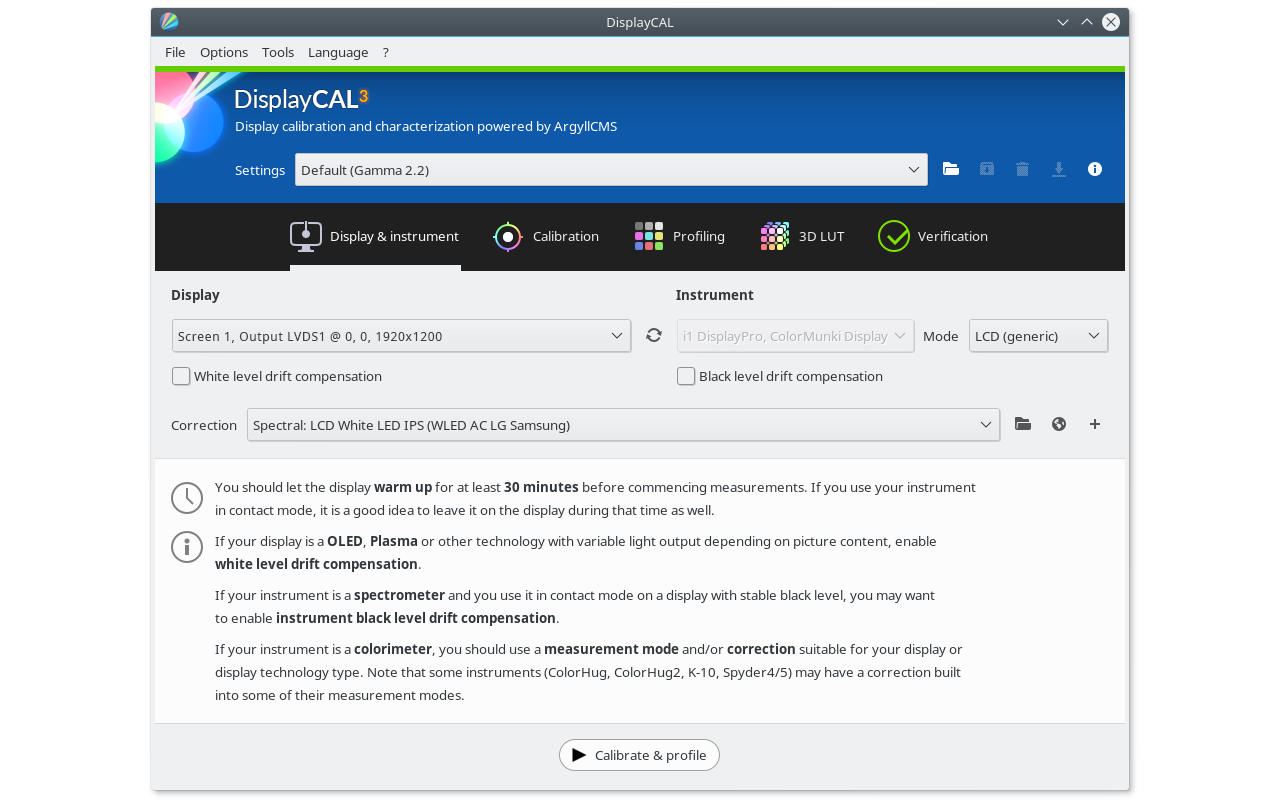
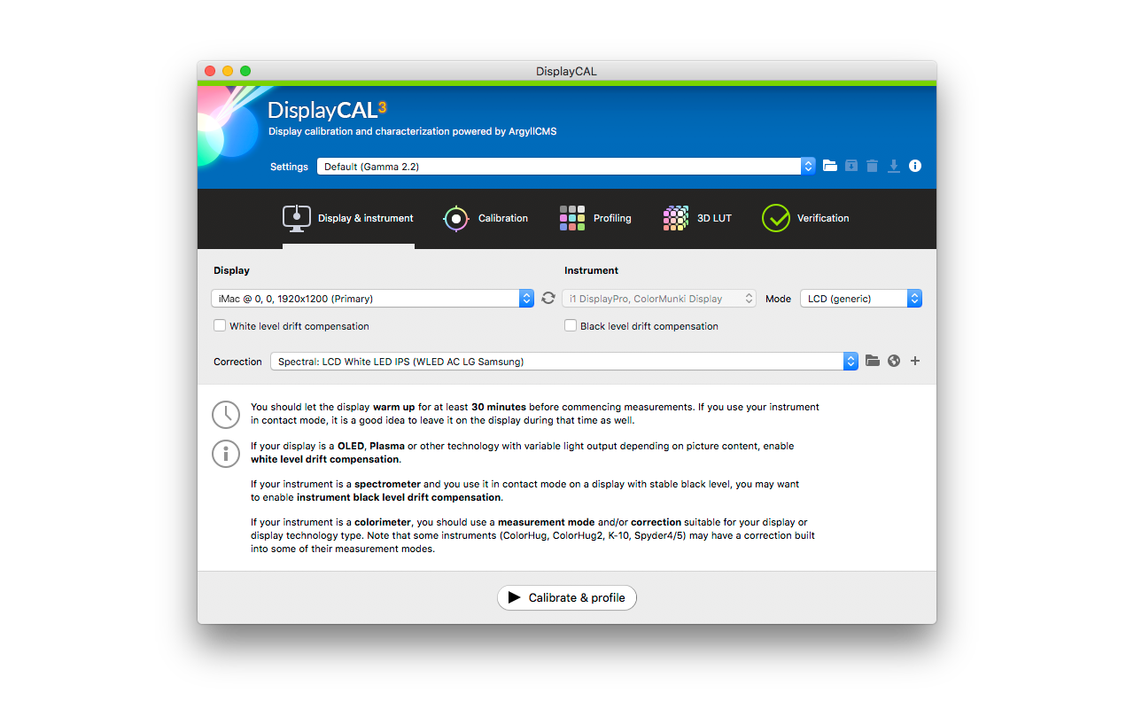
Display & instrument settings
Calibration settings
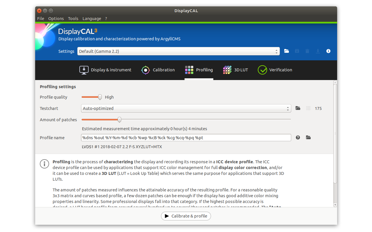
Profiling settings
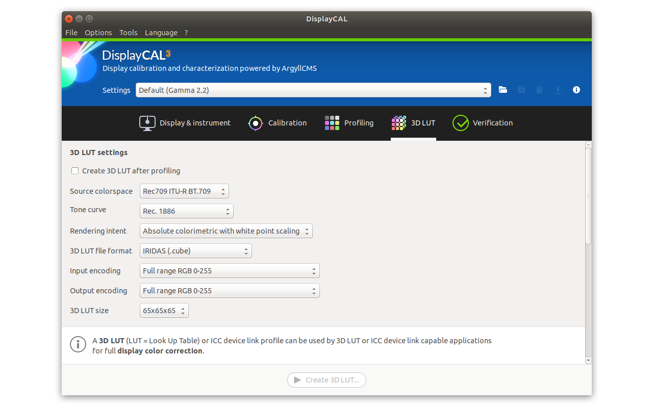
3D LUT settings
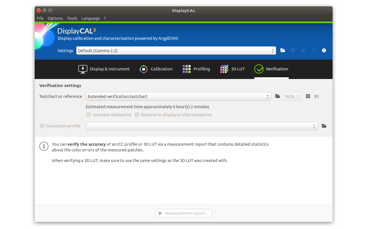
Verification settings
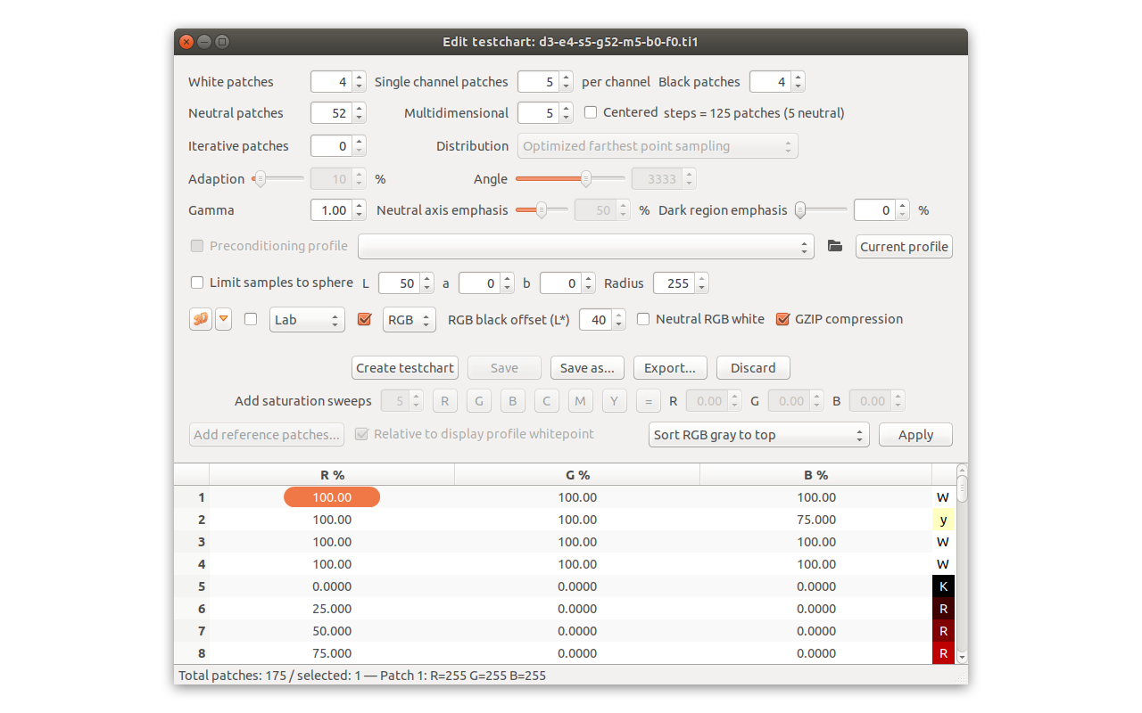
Testchart editor
Display adjustment
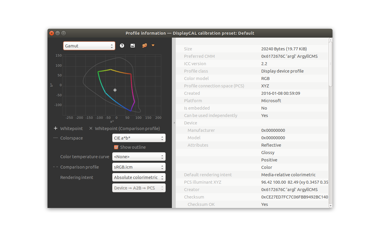
Profile information
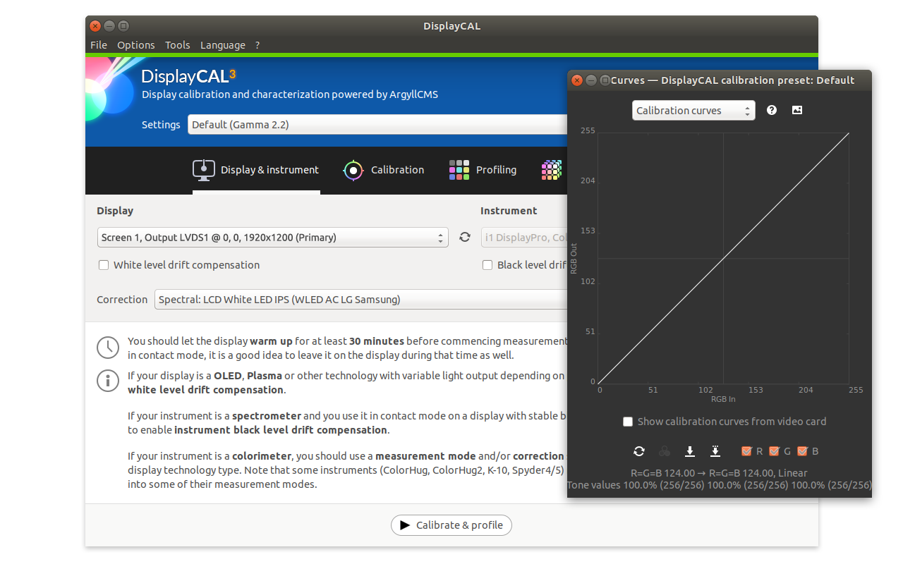
Calibration curves
KDE5
Mac OS X
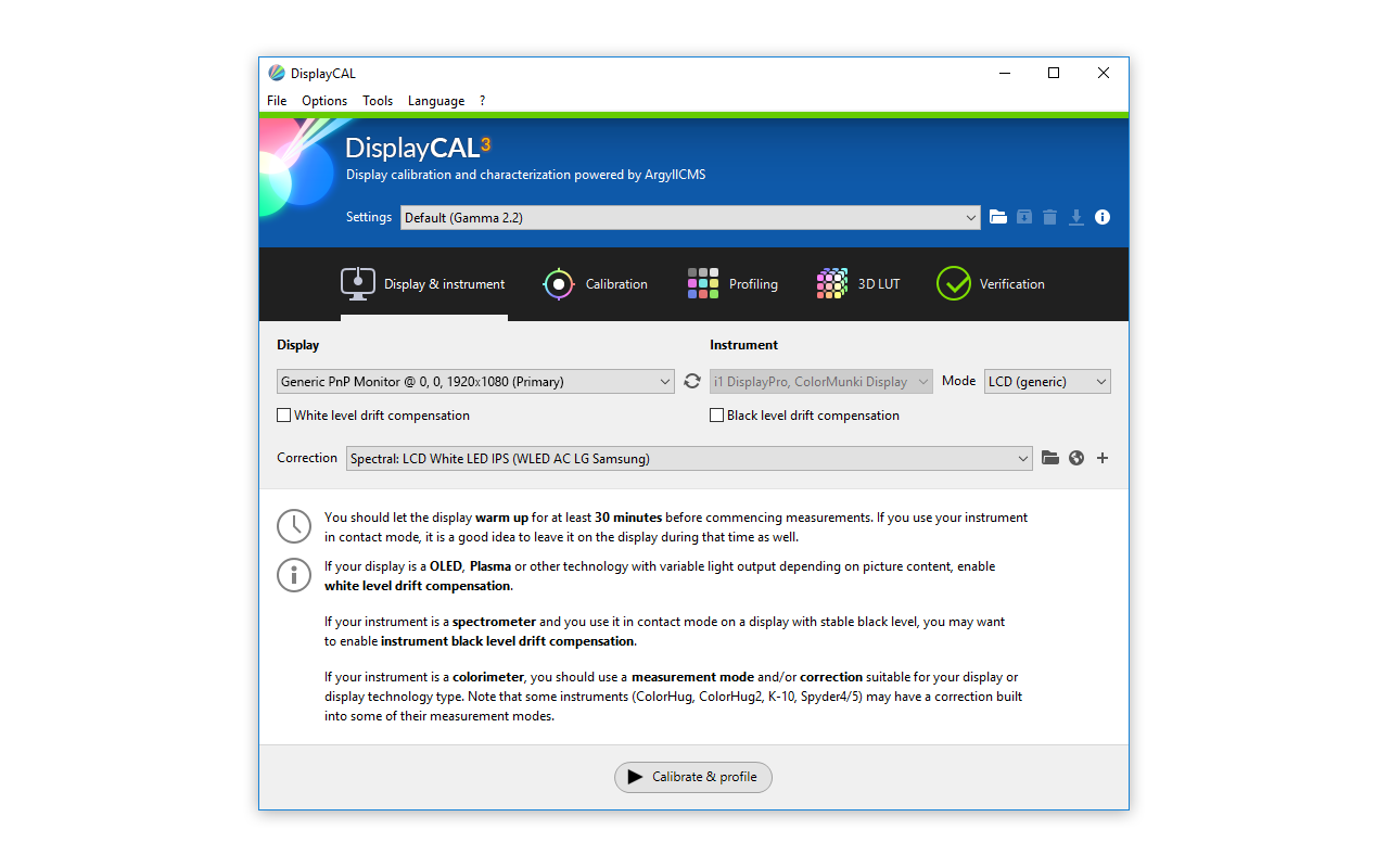
Windows 10
Disclaimer
This program is free software; you can redistribute it and/or modify it under the terms of the GNU General Public License as published by the Free Software Foundation; either version 3 of the License, or (at your option) any later version.
This program is distributed in the hope that it will be useful, but WITHOUT ANY WARRANTY; without even the implied warranty of MERCHANTABILITY or FITNESS FOR A PARTICULAR PURPOSE. See the GNU General Public License for more details.
DisplayCAL is written in Python and uses the 3rd-party packages NumPy, wxPython (GUI[4] toolkit), Certifi, PyGObject or dbus-python for Linux (required for Wayland support with colord), as well as Python extensions for Windows, comtypes and the Python WMI module to provide Windows-specific functionality. Other minor dependencies include faulthandler, psutil, PyChromecast and pyglet (macOS/Windows) or libSDL2 (Linux). It makes extensive use of and depends on functionality provided by ArgyllCMS. The build system to create standalone executables additionally uses py2app on Mac OS X or py2exe on Windows. All of these software packages are © by their respective authors.
Get DisplayCAL
-
For Linux
Native packages for several distributions are available via openSUSE Build Service:
- Arch Linux x86_64
- CentOS 7 x86_64
- Debian 8 (Jessie) x86 | x86_64
- Debian 9 (Stretch) x86 | x86_64
- Debian 10 (Buster) x86 | x86_64
- Fedora 29 x86_64
- Fedora 30 x86_64
- Fedora 31 x86_64
- Mageia 6 x86 | x86_64
- Mageia 7 x86_64
- openSUSE Leap 15.0 x86_64
- openSUSE Leap 15.1 x86_64
- openSUSE Factory x86_64
- openSUSE Tumbleweed x86_64
- Raspbian 9 armv7l
- Raspbian 10 armv7l
- Ubuntu 16.04 (Xenial) x86 | x86_64
- Ubuntu 18.04 (Bionic) x86 | x86_64
- Ubuntu 19.04 (Disco) x86_64
- Ubuntu 19.10 (Eoan) x86_64
Packages made for older distributions may work on newer distributions as long as nothing substantial has changed (i.e. Python version). Also there are several distributions out there that are based on one in the above list (e.g. Linux Mint which is based on Ubuntu). This means that packages for that base distribution should also work on derivatives, you just need to know which version the derivative is based upon and pick your download accordingly.
-
For Mac OS X (10.6 or newer)
If you want to verify the integrity of the downloaded file, compare its SHA-256 checksum to that of the respective entry in the SHA-256 checksum list. To obtain the checksum of the downloaded file, run the following command in Terminal:
shasum -a 256 /Users/Your Username/Downloads/DisplayCAL-3.8.9.3.pkg -
For Windows
Installer (recommended) or ZIP archive
If you want to verify the integrity of the downloaded file, compare its SHA-256 checksum to that of the respective entry in the SHA-256 checksum list (case does not matter). To obtain the checksum of the downloaded file, run the following command in a Windows PowerShell command prompt:
get-filehash -a sha256 C:\Users\Your Username\Downloads\DisplayCAL-3.8.9.3-[Setup.exe|win32.zip] -
Source code
You need to have a working Python installation and all requirements.
If you want to verify the integrity of the downloaded file, compare its SHA-256 checksum to that of the respective entry in the SHA-256 checksum list. To obtain the checksum of the downloaded file, run the following command:
Linux:sha256sum /home/Your Username/Downloads/DisplayCAL-3.8.9.3.tar.gz
macOS:shasum -a 256 /Users/Your Username/Downloads/DisplayCAL-3.8.9.3.tar.gz
Windows (PowerShell command prompt):get-filehash -a sha256 C:\Users\Your Username\Downloads\DisplayCAL-3.8.9.3.tar.gzAlternatively, if you don't mind trying out development code, browse the SVN[8] repository of the latest development version (or do a full checkout using
svn checkout svn://svn.code.sf.net/p/dispcalgui/code/trunk displaycal). But please note that the development code might contain bugs or not run at all, or only on some platform(s). Use at your own risk.
Please continue with the Quickstart Guide.
Quickstart guide
This short guide intends to get you up and running quickly, but if you run into a problem, please refer to the full prerequisites and installation sections.
-
Launch DisplayCAL. If it cannot find ArgyllCMS on your computer, it will prompt you to automatically download the latest version or select the location manually.
-
Windows only: If your measurement device is not a ColorMunki Display, i1 Display Pro, Huey, ColorHug, specbos, spectraval or K-10, you need to install an Argyll-specific driver before continuing (the specbos, spectraval and K-10 may require the FTDI virtual COM port driver instead). Select “Instrument” › “Install ArgyllCMS instrument drivers...” from the “Tools” menu. See also “Instrument driver installation under Windows”.
Mac OS X only: If you want to use the HCFR colorimeter, follow the instructions in the “HCFR Colorimeter” section under “Installing ArgyllCMS on Mac OS X” in the ArgyllCMS documentation before continuing.
Connect your measurement device to your computer.
-
Click the small icon with the swirling arrow
 in between the “Display device” and “Instrument” controls to detect connected display devices and instruments. The detected instrument(s) should show up in the “Instrument” dropdown.
If your measurement device is a Spyder2, a popup dialog will show which will let you enable the device. This is required to be able to use the Spyder2 with ArgyllCMS and DisplayCAL.
If your measurement device is a i1 Display 2, i1 Display Pro, ColorMunki Display, DTP94, Spyder2/3/4/5, a popup dialog will show and allow you to import generic colorimeter corrections from the vendor software which may help measurement accuracy on the type of display you're using. After importing, they are available under the “Correction” dropdown, where you can choose one that fits the type of display you have, or leave it at “Auto” if there is no match. Note: Importing from the Spyder4/5 software enables additional measurement modes for that instrument.
-
Click “Calibrate & profile”. That's it!
Feel free to check out the Wiki for guides and tutorials, and refer to the documentation for advanced usage instructions (optional).
Linux only: If you can't access your instrument, choose “Install ArgyllCMS instrument configuration files...” from the “Tools” menu (if that menu item is grayed out, the ArgyllCMS version you're currently using has probably been installed from the distribution's repository and should already be setup correctly for instrument access). If you still cannot access the instrument, try unplugging and reconnecting it, or a reboot. If all else fails, read “Installing ArgyllCMS on Linux: Setting up instrument access” in the ArgyllCMS documentation.
System requirements and other prerequisites
General system requirements
- A recent Linux, macOS (10.6 or newer, recommended 10.7 or newer) or Windows (recommended Windows 7 or newer) operating system.
- “True color” 24 bits per pixel or higher graphics output.
Hardware requirements
- Minimum: 1 GHz single core processor, 1.5 GB RAM, 500 MB free storage space.
- Recommended: 2 GHz dual core processor or better, 4 GB RAM or more, 1 GB free storage space or more.
ArgyllCMS
To use DisplayCAL, you need to download and install ArgyllCMS (1.0 or newer).
Supported instruments
You need one of the supported instruments to make measurements. All instruments supported by ArgyllCMS are also supported by DisplayCAL. For display readings, these currently are:
Colorimeters
- CalMAN X2 (treated as i1 Display 2)
- Datacolor/ColorVision Spyder2
- Datacolor Spyder3 (since ArgyllCMS 1.1.0)
- Datacolor Spyder4 (since ArgyllCMS 1.3.6)
- Datacolor Spyder5 (since ArgyllCMS 1.7.0)
- Datacolor SpyderX (since ArgyllCMS 2.1.0)
- Hughski ColorHug (Linux support since ArgyllCMS 1.3.6, Windows support with newest ColorHug firmware since ArgyllCMS 1.5.0, fully functional Mac OS X support since ArgyllCMS 1.6.2)
- Hughski ColorHug2 (since ArgyllCMS 1.7.0)
- Image Engineering EX1 (since ArgyllCMS 1.8.0)
- Klein K10-A (since ArgyllCMS 1.7.0. The K-1, K-8 and K-10 are also reported to work)
- Lacie Blue Eye (treated as i1 Display 2)
- Sencore ColorPro III, IV & V (treated as i1 Display 1)
- Sequel Imaging MonacoOPTIX/Chroma 4 (treated as i1 Display 1)
- X-Rite Chroma 5 (treated as i1 Display 1)
- X-Rite ColorMunki Create (treated as i1 Display 2)
- X-Rite ColorMunki Smile (since ArgyllCMS 1.5.0)
- X-Rite DTP92
- X-Rite DTP94
- X-Rite/GretagMacbeth/Pantone Huey
- X-Rite/GretagMacbeth i1 Display 1
- X-Rite/GretagMacbeth i1 Display 2/LT (the HP DreamColor/Advanced Profiling Solution versions of the instrument are also reported to work)
- X-Rite i1 Display Pro, ColorMunki Display (since ArgyllCMS 1.3.4. The HP DreamColor, NEC SpectraSensor Pro and SpectraCal C6 versions of the instrument are also reported to work)
Spectrometers
- JETI specbos 1211/1201 (since ArgyllCMS 1.6.0)
- JETI spectraval 1511/1501 (since ArgyllCMS 1.9.0)
- X-Rite ColorMunki Design/Photo (since ArgyllCMS 1.1.0)
- X-Rite/GretagMacbeth i1 Monitor (since ArgyllCMS 1.0.3)
- X-Rite/GretagMacbeth i1 Pro (the EFI ES-1000 version of the instrument is also reported to work)
- X-Rite i1 Pro 2 (since ArgyllCMS 1.5.0)
- X-Rite/GretagMacbeth Spectrolino
- X-Rite i1Studio (since ArgyllCMS 2.0)
If you've decided to buy a color instrument because ArgyllCMS supports it, please let the dealer and manufacturer know that “You bought it because ArgyllCMS supports it”—thanks.
Note that the i1 Display Pro and i1 Pro are very different instruments despite their naming similarities.
Also there are currently (2014-05-20) five instruments (or rather, packages) under the ColorMunki brand, two of which are spectrometers, and three are colorimeters (not all of them being recent offerings, but you should be able to find them used in case they are no longer sold new):
- The ColorMunki Design and ColorMunki Photo spectrometers differ only in the functionality of the bundled vendor software. There are no differences between the instruments when used with ArgyllCMS and DisplayCAL.
- The ColorMunki Display colorimeter is a less expensive version of the i1 Display Pro colorimeter. It comes bundled with a simpler vendor software and has longer measurement times compared to the i1 Display Pro. Apart from that, the instrument appears to be virtually identical.
- The ColorMunki Create and ColorMunki Smile colorimeters are similar hardware as the i1 Display 2 (with the ColorMunki Smile no longer having a built-in correction for CRT but for white LED backlit LCD instead).
Additional requirements for unattended calibration and profiling
When using a spectrometer that is supported by the unattended feature (see below), having to take the instrument off the screen to do a sensor self-calibration again after display calibration before starting the measurements for profiling may be avoided if the menu item “Allow skipping of spectrometer self-calibration” under the “Advanced” sub-menu in the “Options” menu is checked (colorimeter measurements are always unattended because they generally do not require a sensor calibration away from the screen, with the exception of the i1 Display 1).
Unattended calibration and profiling currently supports the following spectrometers in addition to most colorimeters:
- X-Rite ColorMunki Design/Photo
- X-Rite/GretagMacbeth i1 Monitor & Pro
- X-Rite/GretagMacbeth Spectrolino
- X-Rite i1 Pro 2
- X-Rite i1Studio
Be aware you may still be forced to do a sensor calibration if the instrument requires it. Also, please look at the possible caveats.
Additional requirements for using the source code
You can skip this section if you downloaded a package, installer, ZIP archive or disk image of DisplayCAL for your operating system and do not want to run from source.
All platforms:
- Python >= v2.6 <= v2.7.x (2.7.x is the recommended version. Mac OS X users: If you want to compile DisplayCAL's C extension module, it is advisable to first install XCode and then the official python.org Python)
- NumPy
- wxPython GUI[4] toolkit
- Certifi
- psutil (optional but recommended)
- faulthandler (optional)
- PyChromecast (if you want to use a Chromecast device)
Linux:
Windows:
macOS:
Additional requirements for compiling the C extension module
Normally you can skip this section as the source code contains pre-compiled versions of the C extension module that DisplayCAL uses.
Linux:
- GCC and development headers for Python + X11 + Xrandr + Xinerama + Xxf86vm if not already installed, they should be available through your distribution's packaging system
Mac OS X:
- XCode
- py2app if you want to build a standalone executable. On Mac OS X before 10.5, install setuptools first:
sudo python util/ez_setup.py setuptools
Windows:
- a C-compiler (e.g. MS Visual C++ Express or MinGW. If you're using the official python.org Python 2.6 or later I'd recommend Visual C++ Express as it works out of the box)
- py2exe if you want to build a standalone executable
Running directly from source
After satisfying all additional requirements for using the source code, you can simply run any of the included .pyw files from a terminal, e.g. python2 DisplayCAL.pyw, or install the software so you can access it via your desktop's application menu with python2 setup.py install. Run python2 setup.py --help to view available options.
One-time setup instructions for source code checked out from SVN:
Run python2 setup.py to create the version file so you don't see the update popup at launch.
If the pre-compiled extension module that is included in the sources does not work for you (in that case you'll notice that the movable measurement window's size does not closely match the size of the borderless window generated by ArgyllCMS during display measurements) or you want to re-build it unconditionally, run python2 setup.py build_ext -i to re-build it from scratch (you need to satisfy the requirements for compiling the C extension module first).
Installation
Instrument driver installation under Windows
You only need to install the Argyll-specific driver if your measurement device is not a ColorMunki Display, i1 Display Pro, Huey, ColorHug, specbos, spectraval or K-10 (the latter two may require the FTDI virtual COM port driver instead).
To automatically install the Argyll-specific driver that is needed to use some instruments, launch DisplayCAL and select “Instrument” › “Install ArgyllCMS instrument drivers...” from the “Tools” menu. Alternatively, follow the manual instructions below.
If you are using Windows 8, 8.1, or 10, you need to disable driver signature enforcement before you can install the driver. If Secure Boot is enabled in the UEFI[12] setup, you need to disable it first. Refer to your mainboard or firmware manual how to go about this. Usually entering the firmware setup requires holding the DEL key when the system starts booting.
Method 1: Disable driver signature enforcement temporarily
- Windows 8/8.1: Go to “Settings” (hover the lower right corner of the screen, then click the gear icon) and select “Power” (the on/off icon).
Windows 10: Click the “Power” button in the start menu. - Hold the SHIFT key down and click “Restart”.
- Select “Troubleshoot” → “Advanced Options” → “Startup Settings” → “Restart”
- After reboot, select “Disable Driver Signature Enforcement” (number 7 on the list)
Method 2: Disable driver signature enforcement permanently
- Open an elevated command prompt. Search for “Command Prompt” in the Windows start menu, right-click and select “Run as administrator”
- Run the following command:
bcdedit /set loadoptions DDISABLE_INTEGRITY_CHECKS - Run the following command:
bcdedit /set TESTSIGNING ON - Reboot
To install the Argyll-specific driver that is needed to use some instruments, launch Windows' Device Manager and locate the instrument in the device list. It may be underneath one of the top level items. Right click on the instrument and select “Update Driver Software...”, then choose “Browse my computer for driver software”, “Let me pick from a list of device drivers on my computer”, “Have Disk...”, browse to the Argyll_VX.X.X\usb folder, open the ArgyllCMS.inf file, click OK, and finally confirm the Argyll driver for your instrument from the list.
To switch between the ArgyllCMS and vendor drivers, launch Windows' Device Manager and locate the instrument in the device list. It may be underneath one of the top level items. Right click on the instrument and select “Update Driver Software...”, then choose “Browse my computer for driver software”, “Let me pick from a list of device drivers on my computer” and finally select the desired driver for your instrument from the list.
Linux package (.deb/.rpm)
A lot of distributions allow easy installation of packages via the graphical desktop, i.e. by double-clicking the package file's icon. Please consult your distribution's documentation if you are unsure how to install packages.
If you cannot access your instrument, first try unplugging and reconnecting it, or a reboot. If that doesn't help, read “Installing ArgyllCMS on Linux: Setting up instrument access”.
Mac OS X
Use the Installer Package to install DisplayCAL to your “Applications” folder. Afterwards open the “DisplayCAL” folder in your “Applications” folder and drag DisplayCAL's icon to the dock if you want easy access.
If you want to use the HCFR colorimeter under Mac OS X, follow the instructions under “installing ArgyllCMS on Mac OS X” in the ArgyllCMS documentation.
Windows (Installer)
Launch the installer which will guide you trough the required setup steps.
If your measurement device is not a ColorMunki Display, i1 Display Pro, Huey, ColorHug, specbos, spectraval or K-10, you need to install an Argyll-specific driver (the specbos, spectraval and K-10 may require the FTDI virtual COM port driver instead). See “Instrument driver installation under Windows”.
Windows (ZIP archive)
Unpack and then simply run DisplayCAL from the created folder.
If your measurement device is not a ColorMunki Display, i1 Display Pro, Huey, ColorHug, specbos, spectraval or K-10, you need to install an Argyll-specific driver (the specbos, spectraval and K-10 may require the FTDI virtual COM port driver instead). See “Instrument driver installation under Windows”.
Source code (all platforms)
See the “Prerequisites” section to run directly from source.
Starting with DisplayCAL 0.2.5b, you can use standard distutils/setuptools commands with setup.py to build, install, and create packages. sudo python setup.py install will compile the extension modules and do a standard installation. Run python setup.py --help or python setup.py --help-commands for more information. A few additional commands and options which are not part of distutils or setuptools (and thus do not appear in the help) are also available:
Additional setup commands
0install- Create/update 0install feeds and create Mac OS X application bundles to run those feeds.
appdata- Create/update AppData file.
bdist_appdmg(Mac OS X only)- Creates a DMG of previously created (by the py2app or bdist_standalone commands) application bundles, or if used together with the
0installcommand. bdist_pkg(Mac OS X only)- Creates an Installer Package (.pkg) of previously created (by the py2app or bdist_standalone commands) application bundles.
bdist_deb(Linux/Debian-based)- Create an installable Debian (.deb) package, much like the standard distutils command bdist_rpm for RPM packages. Prerequisites:
You first need to install alien and rpmdb, create a dummy RPM database via
sudo rpmdb --initdb, then edit (or create from scratch) the setup.cfg (you can have a look at misc/setup.ubuntu9.cfg for a working example). Under Ubuntu, running utils/dist_ubuntu.sh will automatically use the correct setup.cfg. If you are using Ubuntu 11.04 or any other debian-based distribution which has Python 2.7 as default, you need to edit /usr/lib/python2.7/distutils/command/bdist_rpm.py, and change the lineinstall_cmd = ('%s install -O1 --root=$RPM_BUILD_ROOT 'toinstall_cmd = ('%s install --root=$RPM_BUILD_ROOT 'by removing the-O1flag. Also, you need to change /usr/lib/rpm/brp-compress to do nothing (e.g. change the file contents toexit 0, but don't forget to create a backup copy first) otherwise you will get errors when building. bdist_pyi- An alternative to
bdist_standalone, which uses PyInstaller instead of bbfreeze/py2app/py2exe. bdist_standalone- Creates a standalone application that does not require a Python installation. Uses bbfreeze on Linux, py2app on Mac OS X and py2exe on Windows. setup.py will try and automatically download/install these packages for you if they are not yet installed and if not using the --use-distutils switch. Note: On Mac OS X, older versions of py2app (before 0.4) are not able to access files inside python “egg” files (which are basically ZIP-compressed folders). Setuptools, which is needed by py2app, will normally be installed in “egg” form, thus preventing those older py2app versions from accessing its contents. To fix this, you need to remove any installed setuptools-<version>-py<python-version>.egg files from your Python installation's site-packages directory (normally found under
/Library/Frameworks/Python.framework/Versions/Current/lib). Then, runsudo python util/ez_setup.py -Z setuptoolswhich will install setuptools unpacked, thus allowing py2app to acces all its files. This is no longer an issue with py2app 0.4 and later. buildservice- Creates control files for openSUSE Build Service (also happens implicitly when invoking
sdist). finalize_msi(Windows only)- Adds icons and start menu shortcuts to the MSI installer previously created with
bdist_msi. Successful MSI creation needs a patched msilib (additional information). inno(Windows only)- Creates Inno Setup scripts which can be used to compile setup executables for standalone applications generated by the
py2exeorbdist_standalonecommands and for 0install. purge- Removes the
buildandDisplayCAL.egg-infodirectories including their contents. purge_dist- Removes the
distdirectory and its contents. readme- Creates README.html by parsing misc/README.template.html and substituting placeholders like date and version numbers.
uninstall- Uninstalls the package. You can specify the same options as for the
installcommand.
Additional setup options
--cfg=<name>- Use an alternate setup.cfg, e.g. tailored for a given Linux distribution. The original setup.cfg is backed up and restored afterwards. The alternate file must exist as misc/setup.<name>.cfg
-n,--dry-run- Don't actually do anything. Useful in combination with the uninstall command to see which files would be removed.
--skip-instrument-configuration-files- Skip installation of udev rules and hotplug scripts.
--skip-postinstall- Skip post-installation on Linux (an entry in the desktop menu will still be created, but may not become visible until logging out and back in or rebooting) and Windows (no shortcuts in the start menu will be created at all).
--stability=stable | testing | developer | buggy | insecure- Set the stability for the readme and/or implementation that is added/updated via the
0installcommand. --use-distutils- Force setup to use distutils (default) instead of setuptools. This is useful in combination with the bdist* commands, because it will avoid an artificial dependency on setuptools. This is actually a switch, use it once and the choice is remembered until you specify the
--use-setuptoolsswitch (see next paragraph). --use-setuptools- Force setup to try and use setuptools instead of distutils. This is actually a switch, use it once and the choice is remembered until you specify the
--use-distutilsswitch (see above).
Instrument-specific setup
If your measurement device is a i1 Display 2, i1 Display Pro, ColorMunki Display, DTP94, Spyder2/3/4/5, you'll want to import the colorimeter corrections that are part of the vendor software packages, which can be used to better match the instrument to a particular type of display. Note: The full range of measurement modes for the Spyder4/5 are also only available if they are imported from the Spyder4/5 software.
Choose “Import colorimeter corrections from other display profiling software...” from DisplayCAL's “Tools” menu.
If your measurement device is a Spyder2, you need to enable it to be able to use it with ArgyllCMS and DisplayCAL. Choose “Enable Spyder2 colorimeter...” from DisplayCAL's “Tools” menu.
Basic concept of display calibration and profiling
If you have previous experience, skip ahead. If you are new to display calibration, here is a quick outline of the basic concept.
First, the display behavior is measured and adjusted to meet
user-definable target characteristics, like brightness, gamma and white point.
This step is generally referred to as calibration. Calibration is done by
adjusting the monitor controls, and the output of the graphics card (via
calibration curves, also sometimes called video LUT[7] curves—please don't confuse these with LUT profiles, the differences are explained here) to get as
close as possible to the chosen target.
To meet the user-defined target characteristics, it is generally advisable to
get as far as possible by using the monitor controls, and only thereafter by
manipulating the output of the video card via calibration curves, which are loaded into the video card gamma table, to get the best
results.
Second, the calibrated displays response is measured and an ICC[5] profile describing it is created.
Optionally and for convenience purposes, the calibration is stored in the profile, but both still need to be used together to get correct results. This can lead to some ambiguity, because loading the calibration curves from the profile is generally the responsibility of a third party utility or the OS, while applications using the profile to do color transforms usually don't know or care about the calibration (they don't need to). Currently, the only OS that applies calibration curves out-of-the-box is Mac OS X (under Windows 7 or later you can enable it, but it's off by default and doesn't offer the same high precision as the DisplayCAL profile loader)—for other OS's, DisplayCAL takes care of creating an appropriate loader.
Even non-color-managed applications will benefit from a loaded calibration because it is stored in the graphics card—it is “global”. But the calibration alone will not yield accurate colors—only fully color-managed applications will make use of display profiles and the necessary color transforms.
Regrettably there are several image viewing and editing applications that only implement half-baked color management by not using the system's display profile (or any display profile at all), but an internal and often unchangeable “default” color space like sRGB, and sending output unaltered to the display after converting to that default colorspace. If the display's actual response is close to sRGB, you might get pleasing (albeit not accurate) results, but on displays which behave differently, for example wide-color-gamut displays, even mundane colors can get a strong tendency towards neon.
A note about colorimeters, displays and DisplayCAL
Colorimeters need a correction in hardware or software to obtain correct measurements from different types of displays (please also see “Wide Gamut Displays and Colorimeters” on the ArgyllCMS website for more information). The latter is supported when using ArgyllCMS >= 1.3.0, so if you own a display and colorimeter which has not been specifically tuned for this display (i.e. does not contain a correction in hardware), you can apply a correction that has been calculated from spectrometer measurements to help better measure such a screen.
You need a spectrometer in the first place to do the necessary measurements to create such a correction, or you may query DisplayCAL's Colorimeter Corrections Database, and there's also a list of contributed colorimeter correction files on the ArgyllCMS website—please note though that a matrix created for one particular instrument/display combination may not work well for different instances of the same combination because of display manufacturing variations and generally low inter-instrument agreement of most older colorimeters (with the exception of the DTP94), newer devices like the i1 Display Pro/ColorMunki Display seem to be less affected by this.
Starting with DisplayCAL 0.6.8, you can also import generic corrections from some profiling softwares by choosing the corresponding item in the “Tools” menu.
If you buy a screen bundled with a colorimeter, the instrument may have been matched to the screen in some way already, so you may not need a software correction in that case.
Special note about the X-Rite i1 Display Pro, ColorMunki Display and Spyder4/5 colorimeters
These instruments greatly reduce the amount of work needed to match them to a display because they contain the spectral sensitivities of their filters in hardware, so only a spectrometer reading of the display is needed to create the correction (in contrast to matching other colorimeters to a display, which needs two readings: One with a spectrometer and one with the colorimeter).
That means anyone with a particular screen and a spectrometer can create a special Colorimeter Calibration Spectral Set (.ccss) file of that screen for use with those colorimeters, without needing to actually have access to the colorimeter itself.
Usage
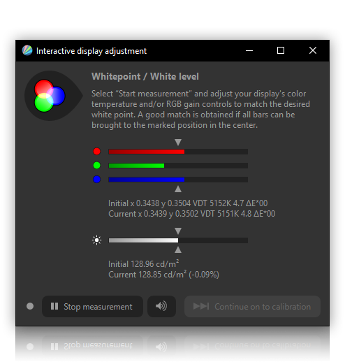
Through the main window, you can choose your settings. When running calibration measurements, another window will guide you through the interactive part of display adjustment.
Settings file
Here, you can load a preset, or a calibration (.cal) or ICC profile (.icc / .icm) file from a previous
run. This will set options to
those stored in the file. If the file contains only a subset of settings, the other options will automatically be reset to defaults (except the 3D LUT settings, which won't be reset if the settings file doesn't contain 3D LUT settings, and the verification settings which will never be reset automatically).
If a calibration file or profile is loaded in this way, its name will
show up here to indicate that the settings reflect those in the file.
Also, if a calibration is present it can be used as the base when “Just Profiling”.
The chosen settings file will stay selected as long as you do not change any of the
calibration or profiling settings, with one exception: When a .cal file with the same base name as the settings file
exists in the same directory, adjusting the quality and profiling controls will not cause unloading of the settings file. This allows you to use an existing calibration with new profiling settings for “Just Profiling”, or to update an existing calibration with different quality and/or profiling settings. If you change settings in other situations, the file will get unloaded (but current settings will be retained—unloading just happens to remind you that the settings no longer match those in the file), and current display profile's calibration curves will be restored (if present, otherwise they will reset to linear).
When a calibration file is selected, the “Update calibration” checkbox will become available, which takes less time than a calibration from scratch. If a ICC[5] profile is selected, and a calibration file with the same base name exists in the same directory, the profile will be updated with the new calibration. Ticking the “Update calibration” checkbox will gray out all options as well as the “Calibrate & profile” and “Just profile” buttons, only the quality level will be changeable.
Predefined settings (presets)
Starting with DisplayCAL v0.2.5b, predefined settings for several use cases are selectable in the settings dropdown. I strongly recommend to NOT view these presets as the solitary “correct” settings you absolutely should use unmodified if your use case matches their description. Rather view them as starting points, from where you can work towards your own, optimized (in terms of your requirements, hardware, surroundings, and personal preference) settings.
Why has a default gamma of 2.2 been chosen for some presets?
Many displays, be it CRT, LCD, Plasma or OLED, have a default response characteristic close to a gamma of approx. 2.2-2.4 (for CRTs, this is the actual native behaviour; and other technologies typically try to mimic CRTs). A target response curve for calibration that is reasonably close to the native response of a display should help to minimize calibration artifacts like banding, because the adjustments needed to the video card's gamma tables via calibration curves will not be as strong as if a target response farther away from the display's native response had been chosen.
Of course, you can and should change the calibration response curve to a value suitable for your own requirements. For example, you might have a display that offers hardware calibration or gamma controls, that has been internally calibrated/adjusted to a different response curve, or your display's response is simply not close to a gamma of 2.2 for other reasons. You can run “Report on uncalibrated display device” from the “Tools” menu to measure the approximated overall gamma among other info.
Tabs
The main user interface is divided into tabs, with each tab containing a sub-set of settings. Not all tabs may be available at any given time. Unavailable tabs will be grayed out.
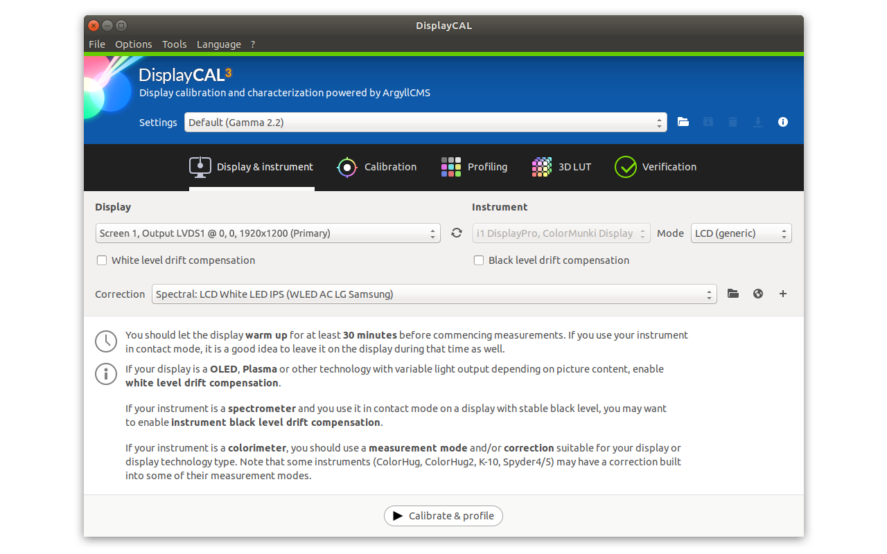
Choosing the display to calibrate and the measurement device
After connecting the instrument, click the small icon with the swirling arrow in between the “Display device” and “Instrument” controls to detect connected display devices and instruments.
Choosing a display device
Directly connected displays will appear at the top of the list as entries in the form “Display Name/Model @ x, y, w, h” with x, y, w and h being virtual screen coordinates depending on resolution and DPI settings. Apart from those directly connected displays, a few additional options are also available:
- Web @ localhost
-
Starts a standalone web server on your machine, which then allows a local or remote web browser to display the color test patches, e.g. to calibrate/profile a smartphone or tablet computer.
Note that if you use this method of displaying test patches, then colors will be displayed with 8 bit per component precision, and any screen-saver or power-saver will not be automatically disabled. You will also be at the mercy of any color management applied by the web browser, and may have to carefully review and configure such color management.
- madVR
-
Causes test patches to be displayed using the madVR Test Pattern Generator (madTPG) application which comes with the madVR video renderer (only available for Windows, but you can connect via local network from Linux and Mac OS X). Note that while you can adjust the test pattern configuration controls in madTPG itself, you should not normally alter the “disable videoLUT” and “disable 3D LUT” controls, as these will be set appropriately automatically when doing measurements.
Note that if you want to create a 3D LUT for use with madVR, there is a “Video 3D LUT for madVR” preset available under “Settings” that will not only configure DisplayCAL to use madTPG, but also setup the correct 3D LUT format and encoding for madVR.
- Prisma
-
The Q, Inc./Murideo Prisma is a video processor and combined pattern generator/3D LUT holder accessible over the network.
Note that if you want to create a 3D LUT for use with a Prisma, there is a “Video 3D LUT for Prisma” preset available under “Settings” that will not only configure DisplayCAL to use a Prisma, but also setup the correct 3D LUT format and encoding.
Also note that the Prisma has 1 MB of internal memory for custom LUT storage, which is enough for around 15 17x17x17 LUTs. You may occasionally need to enter the Prisma's administrative interface via a web browser to delete old LUTs to make space for new ones.
- Resolve
-
Allows you to use the built-in pattern generator of DaVinci Resolve video editing and grading software, which is accessible over the network or on the local machine. The way this works is that you start a calibration or profiling run in DisplayCAL, position the measurement window and click “Start measurement”. A message “Waiting for connection on IP:PORT” should appear. Note the IP and port numbers. In Resolve, switch to the “Color” tab and then choose “Monitor calibration”, “CalMAN” in the “Color” menu (Resolve version 11 and earlier) or the “Workspace” menu (Resolve 12).
Enter the IP address in the window that opens (port should already be filled) and click “Connect” (if Resolve is running on the same machine as DisplayCAL, enterlocalhostor127.0.0.1instead). The position of the measurement window you placed earlier will be mimicked on the display you have connected via Resolve.Note that if you want to create a 3D LUT for use with Resolve, there is a “Video 3D LUT for Resolve” preset available under “Settings” that will not only configure DisplayCAL to use Resolve, but also setup the correct 3D LUT format and encoding.
Note that if you want to create a 3D LUT for a display that is directly connected (e.g. for Resolve's GUI viewer), you should not use the Resolve pattern generator, and select the actual display device instead which will allow for quicker measurements (Resolve's pattern generator has additional delay).
- Untethered
-
See untethered display measurements. Please note that the untethered mode should generally only be used if you've exhausted all other options.
Choosing a measurement mode
Some instruments may support different measurement modes for different types of display devices. In general, there are two base measurement modes: “LCD” and “Refresh” (e.g. CRT and Plasma are refresh-type displays). Some instruments like the Spyder4/5 and ColorHug support additional measurement modes, where a mode is coupled with a predefined colorimeter correction (in that case, the colorimeter correction dropdown will automatically be set to “None”).
Variations of these measurement modes may be available depending on the instrument: “Adaptive” measurement mode for spectrometers uses varying integration times (always used by colorimeters) to increase accuracy of dark readings. “HiRes” turns on high resolution spectral mode for spectrometers like the i1 Pro, which may increase the accuracy of measurements.
Drift compensation during measurements (only available if using ArgyllCMS >= 1.3.0)
White level drift compensation tries to counter luminance changes of a warming up display device. For this purpose, a white test patch is measured periodically, which increases the overall time needed for measurements.
Black level drift compensation tries to counter measurement deviations caused by black calibration drift of a warming up measurement device. For this purpose, a black test patch is measured periodically, which increases the overall time needed for measurements. Many colorimeters are temperature stabilised, in which case black level drift compensation should not be needed, but spectrometers like the i1 Pro or ColorMunki Design/Photo/i1Studio are not temperature compensated.
Override display update delay (only available if using ArgyllCMS >= 1.5.0, only visible if “Show advanced options” in the “Options” menu is enabled)
Normally a delay of 200 msec is allowed between changing a patch color in software, and that change appearing in the displayed color itself. For some instuments (i.e. i1 Display Pro, ColorMunki Display, i1 Pro, ColorMunki Design/Photo/i1Studio, Klein K10-A) ArgyllCMS will automatically measure and set an appropriate update delay during instrument calibration. In rare situations this delay may not be sufficient (ie. some TV's with extensive image processing features turned on), and a larger delay can be set here.
Override display settle time multiplier (only available if using ArgyllCMS >= 1.7.0, only visible if “Show advanced options” in the “Options” menu is enabled)
Normally the display technology type determines how long is allowed between when a patch color change appears on the display, and when that change has settled down, and as actually complete within measurement tolerance. A CRT or Plasma display for instance, can have quite a long settling delay due to the decay characteristics of the phosphor used, while an LCD can also have a noticeable settling delay due to the liquid crystal response time and any response time enhancement circuit (instruments without a display technology type selection such as spectrometers assume a worst case).
The display settle time multiplier allows the rise and fall times of the model to be scaled to extend or reduce the settling time. For instance, a multiplier of 2.0 would double the settling time, while a multiplier of 0.5 would halve it.
Output levels (only visible if “Show advanced options” in the “Options” menu is enabled)
The default value of “Auto” detects the correct output levels automatically during measurements. This usually takes a few seconds. If you know the correct output levels for the selected display, you can set it here.
Full field pattern insertion (only for select pattern generators, only visible if “Show advanced options” in the “Options” menu is enabled)
Full field pattern insertion can help with displays that employ ASBL (automatic static brightness limiting), like some types of OLED and HDR displays. A full field pattern is shown every few seconds (the minimum interval can be set with the respective control) for a given duration, at a given signal level, if this option is enabled.
Choosing a colorimeter correction for a particular display
This can improve a colorimeters accuracy for a particular type of display, please also see “A note about colorimeters, displays and DisplayCAL”. You can import generic matrices from some other display profiling softwares, as well as check the online Colorimeter Corrections Database for a match of your display/instrument combination (click the small globe next to the correction dropdown)—please note though that all colorimeter corrections in the online database have been contributed by various users, and their usefulness to your particular situation is up to you to evaluate: They may or may not improve the absolute accuracy of your colorimeter with your display.
Please note this option is only available if using ArgyllCMS >= 1.3.0 and a colorimeter.
Colorimeter correction information
For correction matrices, a visual simulation of the effect of the correction will be shown (“flower”). Note that this is not meant to be color accurate, but give you a rough idea about the impact on the measurements of your colorimeter. The six outer circles of primary and secondary colors (clockwise: green, yellow, red, magenta, blue, cyan) and center white circle all have an outer part as well as a smaller inner area. The outer part of each circle represents what the colorimeter would “see” (i.e. measure) without the correction, the inner part of each circle represents the corrected result.
Below this visual representation you will find the matrix values, as well as optional further information, like the reference instrument or source used, the method used to create the correction (“perceptual” or “minimize xy chromaticity difference”), as well as the average and maximum fit error (the lower the fit error, the better the corrected instrument should match the reference instrument).
For spectral samples, the respective spectra will be shown along with information about the reference spectrometer used, as well as the resolution and range in nm (nanometer). You can toggle between the spectral graph and a CIE 1931 chromaticity diagram using the button at the top, which allows you to see the corresponding xy locations of the spectra in comparison to several common RGB colorspaces (Rec. 709, DCI P3, Adobe RGB and Rec. 2020).
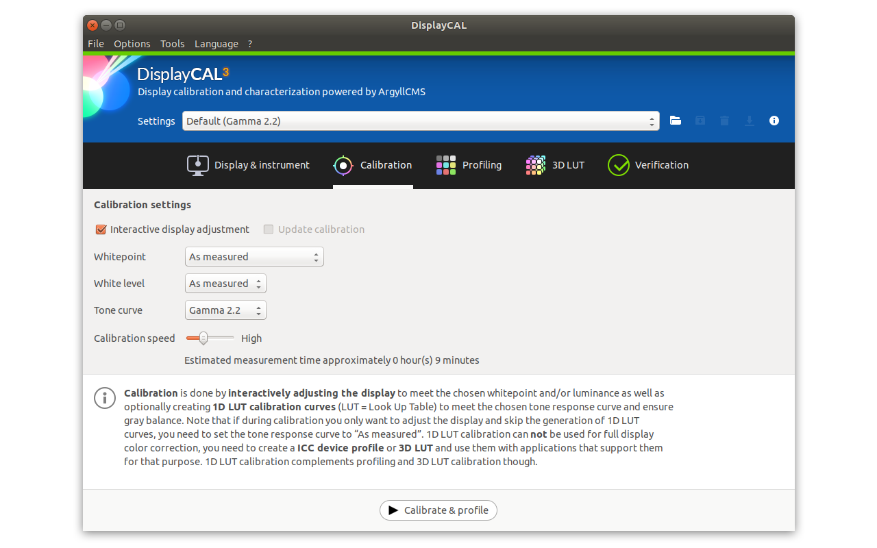
Calibration settings
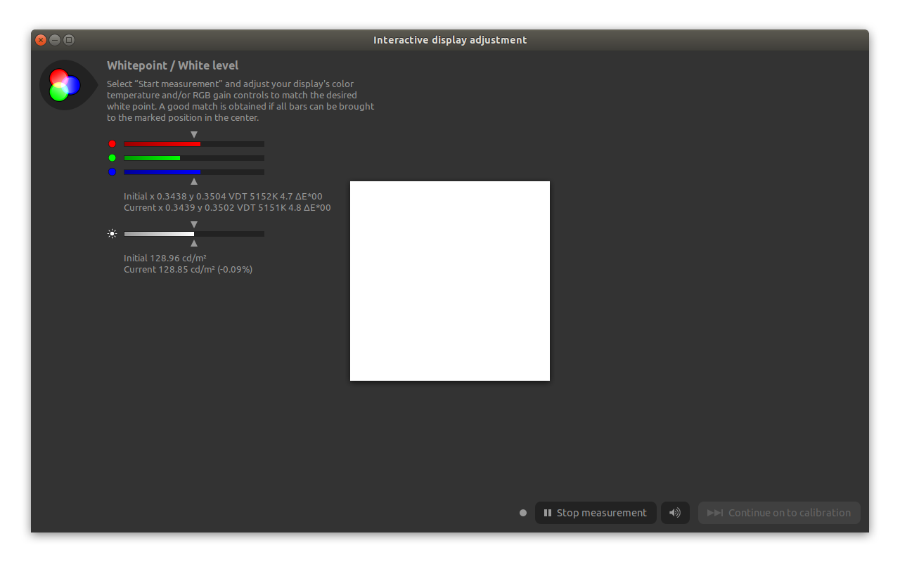
- Interactive display adjustment
- Turning this off skips straight to calibration or profiling measurements instead of giving you the opportunity to alter the display's controls first. You will normally want to keep this checked, to be able to use the controls to get closer to the chosen target characteristics.
- Observer
-
To see this setting, you need to have an instrument that supports spectral readings (i.e. a spectrometer) or spectral sample calibration (e.g. i1 DisplayPro, ColorMunki Display and Spyder4/5), and go into the “Options” menu, and enable “Show advanced options”.
This can be used to select a different colorimetric observer, also known as color matching function (CMF), for instruments that support it. The default is the CIE 1931 standard 2° observer.
Note that if you select anything other than the default 1931 2 degree observer, then the Y values will not be cd/m², due to the Y curve not being the CIE 1924 photopic V(λ) luminosity function.
- White point
-
Allows setting the target white point locus to the equivalent of a daylight or black body spectrum of the given temperature in degrees Kelvin, or as chromaticity co-ordinates. By default the white point target will be the native white of the display, and it's color temperature and delta E to the daylight spectrum locus will be shown during monitor adjustment, and adjustments will be recommended to put the display white point directly on the Daylight locus. If a daylight color temperature is given, then this will become the target of the adjustment, and the recommended adjustments will be those needed to make the monitor white point meet the target. Typical values might be 5000 for matching printed output, or 6500, which gives a brighter, bluer look. A white point temperature different to that native to the display may limit the maximum brightness possible.
A whitepoint other than “As measured” will also be used as the target whitepoint when creating 3D LUTs.
If you want to find out the current uncalibrated whitepoint of your display, you can run “Report on uncalibrated display device” from the “Tools” menu to measure it.
If you want to adjust the whitepoint to the chromaticities of your ambient lighting, or those of a viewing booth as used in prepress and photography, and your measurement device has ambient measuring capability (e.g. like the i1 Pro or i1 Display with their respective ambient measurement heads), you can use the “Measure ambient” button next to the whitepoint settings. If you want to measure ambient lighting, place the instrument upwards, beside the display. Or if you want to measure a viewing booth, put a metamerism-free gray card inside the booth and point the instrument towards it. Further instructions how to measure ambient may be available in your instrument's documentation.
Visual whitepoint editor
The visual whitepoint editor allows visually adjusting the whitepoint on display devices that lack hardware controls as well as match several displays to one another (or a reference). To use it, set the whitepoint to “Chromaticity” and click the visual whitepoint editor button (you can open as many visual whitepoint editors simultaneously as you like, so that e.g. one can be left unchanged as reference, while the other can be adjusted to match said reference). The editor window can be put into a distraction-free fullscreen mode by maximizing it (press ESC to leave fullscreen again). Adjust the whitepoint using the controls on the editor tool pane until you have achieved a visual match. Then, place your instrument on the measurement area and click “Measure”. The measured whitepoint will be set as calibration target.
- White level
-
Set the target brightness of white in cd/m2. If this number cannot be reached, the brightest output possible is chosen, consistent with matching the white point target. Note that many of the instruments are not particularly accurate when assessing the absolute display brightness in cd/m2. Note that some LCD screens behave a little strangely near their absolute white point, and may therefore exhibit odd behavior at values just below white. It may be advisable in such cases to set a brightness slightly less than the maximum such a display is capable of.
If you want to find out the current uncalibrated white level of your display, you can run “Report on uncalibrated display device” from the “Tools” menu to measure it.
- Black level
-
(To see this setting, go into the “Options” menu, and enable “Show advanced options”)
Can be used to set the target brightness of black in cd/m2 and is useful for e.g. matching two different screens with different native blacks to one another, by measuring the black levels on both (i.e. in the “Tools” menu, choose “Report on uncalibrated display”) and then entering the highest measured value. Normally you may want to use native black level though, to maximize contrast ratio. Setting too high a value may also give strange results as it interacts with trying to achieve the target “advertised” tone curve shape. Using a black output offset of 100% tries to minimize such problems.
- Tone curve / gamma
-
The target response curve is normally an exponential curve (output = inputgamma), and defaults to 2.2 (which is close to a typical CRT displays real response). Four pre-defined curves can be used as well: the sRGB colorspace response curve, which is an exponent curve with a straight segment at the dark end and an overall response of approximately gamma 2.2, the L* curve, which is the response of the CIE L*a*b* perceptual colorspace, the Rec. 709 video standard response curve and the SMPTE 240M video standard response curve.
Another possible choice is “As measured”, which will skip video card gamma table (1D LUT) calibration.Note that a real display usually can't reproduce any of the ideal pre-defined curves, since it will have a non-zero black point, whereas all the ideal curves assume zero light at zero input.
For gamma values, you can also specify whether it should be interpreted relative, meaning the gamma value provided is used to set an actual response curve in light of the non-zero black of the actual display that has the same relative output at 50% input as the ideal gamma power curve, or absolute, which allows the actual power to be specified instead, meaning that after the actual displays non-zero black is accounted for, the response at 50% input will probably not match that of the ideal power curve with that gamma value (to see this setting, you have to go into the “Options” menu, and enable “Show advanced options”).
To allow for the non-zero black level of a real display, by default the target curve values will be offset so that zero input gives the actual black level of the display (output offset). This ensures that the target curve better corresponds to the typical natural behavior of displays, but it may not be the most visually even progression from display minimum. This behavior can be changed using the black output offset option (see further below).
Also note that many color spaces are encoded with, and labelled as having a gamma of approximately 2.2 (ie. sRGB, REC 709, SMPTE 240M, Macintosh OS X 10.6), but are actually intended to be displayed on a display with a typical CRT gamma of 2.4 viewed in a darkened environment.
This is because this 2.2 gamma is a source gamma encoding in bright viewing conditions such as a television studio, while typical display viewing conditions are quite dark by comparison, and a contrast expansion of (approx.) gamma 1.1 is desirable to make the images look as intended.
So if you are displaying images encoded to the sRGB standard, or displaying video through the calibration, just setting the gamma curve to sRGB or REC 709 (respectively) is probably not what you want! What you probably want to do, is to set the gamma curve to about gamma 2.4, so that the contrast range is expanded appropriately, or alternatively use sRGB or REC 709 or a gamma of 2.2 but also specify the actual ambient viewing conditions via a light level in Lux, so that an appropriate contrast enhancement can be made during calibration. If your instrument is capable of measuring ambient light levels, then you can do so.
(For in-depth technical information about sRGB, see “A Standard Default Color Space for the Internet: sRGB” at the ICC[5] website for details of how it is intended to be used)If you're wondering what gamma value you should use, you can run “Report on uncalibrated display device” from the “Tools” menu to measure the approximated overall gamma among other info. Setting the gamma to the reported value can then help to reduce calibration artifacts like banding, because the adjustments needed for the video card's gamma table should not be as strong as if a gamma further away from the display's native response was chosen.
- Ambient light level
-
(To see this setting, go into the “Options” menu, and enable “Show advanced options”)
As explained for the tone curve settings, often colors are encoded in a situation with viewing conditions that are quite different to the viewing conditions of a typical display, with the expectation that this difference in viewing conditions will be allowed for in the way the display is calibrated. The ambient light level option is a way of doing this. By default calibration will not make any allowances for viewing conditions, but will calibrate to the specified response curve, but if the ambient light level is entered or measured, an appropriate viewing conditions adjustment will be performed. For a gamma value or sRGB, the original viewing conditions will be assumed to be that of the sRGB standard viewing conditions, while for REC 709 and SMPTE 240M they will be assumed to be television studio viewing conditions.
By specifying or measuring the ambient lighting for your display, a viewing conditions adjustment based on the CIECAM02 color appearance model will be made for the brightness of your display and the contrast it makes with your ambient light levels.Please note your measurement device needs ambient measuring capability (e.g. like the i1 Pro or i1 Display with their respective ambient measurement heads) to measure the ambient light level.
- Black output offset
-
(To see this setting, go into the “Options” menu, and enable “Show advanced options”)
Real displays do not have a zero black response, while all the target response curves do, so this has to be allowed for in some way.
The default way of handling this (equivalent to 100% black output offset) is to allow for this at the output of the ideal response curve, by offsetting and scaling the output values. This defined a curve that will match the responses that many other systems provide and may be a better match to the natural response of the display, but will give a less visually even response from black.
The other alternative is to offset and scale the input values into the ideal response curve so that zero input gives the actual non-zero display response. This ensures the most visually even progression from display minimum, but might be hard to achieve since it is different to the natural response of a display.
A subtlety is to provide a split between how much of the offset is accounted for as input to the ideal response curve, and how much is accounted for at the output, where the degree is 0.0 accounts for it all as input offset, and 100% accounts for all of it as output offset.
- Black point correction
-
(To see this setting, go into the “Options” menu, and enable “Show advanced options”)
Normally dispcal will attempt to make all colors down the neutral axis (R=G=B) have the same hue as the chosen white point. Near the black point, red, green or blue can only be added, not subtracted from zero, so the process of making the near black colors have the desired hue, will lighten them to some extent. For a device with a good contrast ratio or a black point that has nearly the same hue as the white, this is not a problem. If the device contrast ratio is not so good, and the black hue is noticeably different to that of the chosen white point (which is often the case for LCD type displays), this could have a noticeably detrimental effect on an already limited contrast ratio. Here the amount of black point hue correction can be controlled.
By default a factor of 100% will be used, which is usually good for “Refresh”-type displays like CRT or Plasma and also by default a factor of 0% is used for LCD type displays, but you can override these with a custom value between 0% (no correction) to 100% (full correction), or enable automatically setting it based on the measured black level of the display.If less than full correction is chosen, then the resulting calibration curves will have the target white point down most of the curve, but will then cross over to the native or compromise black point.
- Black point correction rate (only available if using ArgyllCMS >= 1.0.4)
-
(To see this setting, go into the “Options” menu, and enable “Show advanced options”)
If the black point is not being set completely to the same hue as the white point (ie. because the factor is less than 100%), then the resulting calibration curves will have the target white point down most of the curve, but will then blend over to the native or compromise black point that is blacker, but not of the right hue. The rate of this blend can be controlled. The default value is 4.0, which results in a target that switches from the white point target to the black, moderately close to the black point. While this typically gives a good visual result with the target neutral hue being maintained to the point where the crossover to the black hue is not visible, it may be asking too much of some displays (typically LCD type displays), and there may be some visual effects due to inconsistent color with viewing angle. For this situation a smaller value may give a better visual result (e.g. try values of 3.0 or 2.0. A value of 1.0 will set a pure linear blend from white point to black point). If there is too much coloration near black, try a larger value, e.g. 6.0 or 8.0.
- Calibration speed
-
(This setting will not apply and be hidden when the tone curve is set to “As measured”)
Determines how much time and effort to go to in calibrating the display. The lower the speed, the more test readings will be done, the more refinement passes will be done, the tighter will be the accuracy tolerance, and the more detailed will be the calibration of the display. The result will ultimately be limited by the accuracy of the instrument, the repeatability of the display and instrument, and the resolution of the video card gamma table entries and digital or analogue output (RAMDAC).
Profiling settings
- Profile quality
- Sets the level of effort and/or detail in the resulting profile. For table based profiles (LUT[7]), it sets the main lookup table size, and hence quality in the resulting profile. For matrix profiles it sets the per channel curve detail level and fitting “effort”.
- Black point compensation (enable “Show advanced options” in the “Options” menu)
-
(Note: This option has no effect if just calibrating and creating a simple curves + matrix profile directly from the calibration data without additional profiling measurements)
This effectively prevents black crush when using the profile, but at the expense of accuracy. It is generally best to only use this option when it is not certain that the applications you are going to use have a high quality color management implementation. For LUT profiles, more sophisticated options exist (i.e. advanced gamut mapping options and use either “Enhance effective resolution of colorimetric PCS[11]-to-device tables”, which is enabled by default, or “Gamut mapping for perceptual intent”, which can be used to create a perceptual table that maps the black point).
- Profile type (enable “Show advanced options” in the “Options” menu)
-
Generally you can differentiate between two types of profiles: LUT[7] based and matrix based.
Matrix based profiles are smaller in filesize, somewhat less accurate (though in most cases smoother) compared to LUT[7] based types, and usually have the best compatibility across CMM[2]s, applications and systems — but only support the colorimetric intent for color transforms. For matrix based profiles, the PCS[11] is always XYZ. You can choose between using individual curves for each channel (red, green and blue), a single curve for all channels, individual gamma values for each channel or a single gamma for all channels. Curves are more accurate than gamma values. A single curve or gamma can be used if individual curves or gamma values degrade the gray balance of an otherwise good calibration.
LUT[7] based profiles are larger in filesize, more accurate (but may sacrifice smoothness), in some cases less compatible (applications might not be able to use or show bugs/quirks with LUT[7] type profiles, or certain variations of them). When choosing a LUT[7] based profile type, advanced gamut mapping options become available which you can use to create perceptual and/or saturation tables inside the profile in addition to the default colorimetric tables which are always created.
L*a*b* or XYZ can be used as PCS[11], with XYZ being recommended especially for wide-gamut displays bacause their primaries might exceed the ICC[5] L*a*b* encoding range (Note: Under Windows, XYZ LUT[7] types are only available in DisplayCAL if using ArgyllCMS >= 1.1.0 because of a requirement for matrix tags in the profile, which are not created by prior ArgyllCMS versions).
As it is hard to verify if the LUT[7] of an combined XYZ LUT[7] + matrix profile is actually used, you may choose to create a profile with a swapped matrix, ie. blue-red-green instead of red-green-blue, so it will be obvious if an application uses the (deliberately wrong) matrix instead of the (correct) LUT because the colors will look very wrong (e.g. everything that should be red will be blue, green will be red, blue will be green, yellow will be purple etc).Note: LUT[7]-based profiles (which contain three-dimensional LUTs) might be confused with video card LUT[7] (calibration) curves (one-dimensional LUTs), but they're two different things. Both LUT[7]-based and matrix-based profiles may include calibration curves which can be loaded into a video card's gamma table hardware.
- Advanced gamut mapping options (enable “Show advanced options” in the “Options” menu)
-
You can choose any of the following options after selecting a LUT profile type and clicking “Advanced...”. Note: The options “Low quality PCS[11]-to-device tables” and “Enhance effective resolution of colorimetric PCS[11]-to-device table” are mutually exclusive.
Low quality PCS[11]-to-device tables
Choose this option if the profile is only going to be used with inverse device-to-PCS[11] gamut mapping to create a DeviceLink or 3D LUT (DisplayCAL always uses inverse device-to-PCS[11] gamut mapping when creating a DeviceLink/3D LUT). This will reduce the processing time needed to create the PCS[11]-to-device tables. Don't choose this option if you want to install or otherwise use the profile.
Enhance effective resolution of colorimetric PCS[11]-to-device table
To use this option, you have to select a XYZ or L*a*b* LUT profile type (XYZ will be more effective). This option increases the effective resolution of the PCS[11] to device colorimetric color lookup table by using a matrix to limit the XYZ space and fill the whole grid with the values obtained by inverting the device-to-PCS[11] table, as well as optionally applies smoothing. If no CIECAM02 gamut mapping has been enabled for the perceptual intent, a simple but effective perceptual table (which is almost identical to the colorimetric table, but maps the black point to zero) will also be generated.
You can also set the interpolated lookup table size. The default “Auto” will use a base 33x33x33 resulution that is increased if needed and provide a good balance between smoothness and accuracy. Lowering the resolution can increase smoothness (at the potential expense of some accuracy), while increasing resolution may make the resulting profile potentially more accurate (at the expense of some smoothness). Note that computation will need a lot of memory (>= 4 GB of RAM recommended to prevent swapping to harddisk) especially at higher resolutions.
See below example images for the result you can expect, where the original image has been converted from sRGB to the display profile. Note though that the particular synthetic image chosen, a “granger rainbow”, exaggerates banding, real-world material is much less likely to show this. Also note that the sRGB blue in the image is actually out of gamut for the specific display used, and the edges visible in the blue gradient for the rendering are a result of the color being out of gamut, and the gamut mapping thus hitting the less smooth gamut boundaries.
Default rendering intent for profile
Sets the default rendering intent. In theory applications could use this, in practice they don't, so changing this setting probably won't have any effect whatsoever.
CIECAM02 gamut mapping
Note: When enabling one of the CIECAM02 gamut mapping options, and the source profile is a matrix profile, then enabling effective resolution enhancement will also influence the CIECAM02 gamut mapping, making it smoother, more accurate and also generated faster as a side-effect.
Normally, profiles created by DisplayCAL only incorporate the colorimetric rendering intent, which means colors outside the display's gamut will be clipped to the next in-gamut color. LUT-type profiles can also have gamut mapping by implementing perceptual and/or saturation rendering intents (gamut compression/expansion). You can choose if and which of those you want by specifying a source profile and marking the appropriate checkboxes. Note that a input, output, display or device colororspace profile should be specified as source, not a non-device colorspace, device link, abstract or named color profile. You can also choose viewing conditions which describe the intended use of both the source and the display profile that is to be generated. An appropriate source viewing condition is chosen automatically based on the source profile type.
An explanation of the available rendering intents can be found in the 3D LUT section “Rendering intent”.
For more information on why a source gamut is needed, see “About ICC profiles and Gamut Mapping” in the ArgyllCMS documentation.
One strategy for getting the best perceptual results with display profiles is as follows: Select a CMYK profile as source for gamut mapping. Then, when converting from another RGB profile to the display profile, use relative colorimetric intent, and if converting from a CMYK profile, use the perceptual intent.
Another approach which especially helps limited-gamut displays is to choose one of the larger (gamut-wise) source profiles you usually work with for gamut mapping, and then always use perceptual intent when converting to the display profile.Please note that not all applications support setting a rendering intent for display profiles and might default to colorimetric (e.g. Photoshop normally uses relative colorimetric with black point compensation, but can use different intents via custom soft proofing settings).
- Testchart file
- You can choose the test patches used when profiling the display here. The default “Auto” optimized setting takes the actual display characteristics into account. You can further increase potential profile accuracy by increasing the number of patches using the slider.
- Patch sequence (enable “Show advanced options” in the “Options” menu)
-
Controls the order in which the patches of a testchart are measured. “Minimize display response delay” is the ArgyllCMS test patch generator default, which should lead to the lowest overall measurement time. The other choices (detailed below) are aimed at potentially dealing better with displays employing ASBL (automatic static brightness limiting) leading to distorted measurements, and should be used together with display white level drift compensation (although overall measurement time will increase somewhat by using either option). If your display doesn't have ASBL issues, there is no need to change this settting.
- Maximize lightness difference will order the patches in such a way that there is the highest possible difference in terms of lightness between patches, while keeping the overall light output relatively constant (but increasing) over time. The lightness of a patch is calculated using sRGB-like relative luminance. This is the recommended setting for dealing with ASBL if you're unsure which choice to make.
- Maximize luma difference will order the patches in such a way that there is the highest possible difference in terms of luma between patches, while keeping the overall luma relatively constant (but increasing) over time. The luma of a patch is calculated from Rec. 709 luma coefficients. The order of the patches will in most cases be quite similar to “Maximize lightness difference”.
- Maximize RGB difference will order the patches in such a way that there is the highest possible difference in terms of the red, green and blue components between patches.
- Vary RGB difference will order the patches in such a way that there is some difference in terms of the red, green and blue components between patches.
Which of the choices works best on your ASBL display depends on how the display detects wether it should reduce light output. If it looks at the (assumed) relative luminance (or luma), then “Maximize lightness difference” or “Maximize luma difference” should work best. If your display is using an RGB instead of YCbCr signal path, then “Maximize RGB difference” or “Vary RGB difference” may produce desired results.
- Testchart editor
-
The provided default testcharts should work well in most situations, but allowing you to create custom charts ensures maximum flexibility when characterizing a display and can improve profiling accuracy and efficiency. See also optimizing testcharts.
Testchart generation options
You can enter the amount of patches to be generated for each patch type (white, black, gray, single channel, iterative and multidimensional cube steps). The iterative algorythm can be tuned if more than zero patches are to be generated. What follows is a quick description of the several available iterative algorythms, with “device space” meaning in this case RGB coordinates, and “perceptual space” meaning the (assumed) XYZ numbers of those RGB coordinates. The assumed XYZ numbers can be influenced by providing a previous profile, thus allowing optimized test point placement.
- Optimized Farthest Point Sampling (OFPS) will optimize the point locations to minimize the distance from any point in device space to the nearest sample point
- Incremental Far Point Distribution incrementally searches for test points that are as far away as possible from any existing points
- Device space random chooses test points with an even random distribution in device space
- Perceptual space random chooses test points with an even random distribution in perceptual space
- Device space filling quasi-random chooses test points with a quasi-random, space filling distribution in device space
- Perceptual space filling quasi-random chooses test points with a quasi-random, space filling distribution in perceptual space
- Device space body centered cubic grid chooses test points with body centered cubic distribution in device space
- Perceptual space body centered cubic grid chooses test points with body centered cubic distribution in perceptual space
You can set the degree of adaptation to the known device characteristics used by the default full spread OFPS algorithm. A preconditioning profile should be provided if adaptation is set above a low level. By default the adaptation is 10% (low), and should be set to 100% (maximum) if a profile is provided. But, if for instance, the preconditioning profile doesn't represent the device behavior very well, a lower adaption than 100% might be appropriate.
For the body centered grid distributions, the angle parameter sets the overall angle that the grid distribution has.
The “Gamma” parameter sets a power-like (to avoid the excessive compression that a real power function would apply) value applied to all of the device values after they are generated. A value greater than 1.0 will cause a tighter spacing of test values near device value 0.0, while a value less than 1.0 will cause a tighter spacing near device value 1.0. Note that the device model used to create the expected patch values will not take into account the applied power, nor will the more complex full spread algorithms correctly take into account the power.
The neutral axis emphasis parameter allows changing the degree to which the patch distribution should emphasise the neutral axis. Since the neutral axis is regarded as the most visually critical area of the color space, it can help maximize the quality of the resulting profile to place more measurement patches in this region. This emphasis is only effective for perceptual patch distributions, and for the default OFPS distribution if the adaptation parameter is set to a high value. It is also most effective when a preconditioning profile is provided, since this is the only way that neutral can be determined. The default value of 50% provides an effect about twice the emphasis of the CIE94 Delta E formula.
The dark region emphasis parameter allows changing the degree to which the patch distribution should emphasis dark region of the device response. Display devices used for video or film reproduction are typically viewed in dark viewing environments with no strong white reference, and typically employ a range of brightness levels in different scenes. This often means that the devices dark region response is of particular importance, so increasing the relative number of sample points in the dark region may improve the balance of accuracy of the resulting profile for video or film reproduction. This emphasis is only effective for perceptual patch distributions where a preconditioning profile is provided. The default value of 0% provides no emphasis of the dark regions. A value somewhere around 15% - 30% is a good place to start for video profile use. A scaled down version of this parameter will be passed on to the profiler. Note that increasing the proportion of dark patches will typically lengthen the time that an instrument takes to read the whole chart. Emphasizing the dark region characterization will reduce the accuracy of measuring and modelling the lighter regions, given a fixed number of test points and profile quality/grid resolution. The parameter will also be used in an analogous way to the “Gamma” value in changing the distribution of single channel, grayscale and multidimensional steps.
The “Limit samples to sphere” option is used to define an L*a*b* sphere to filter the test points through. Only test points within the sphere (defined by it's center and radius) will be in the generated testchart. This can be good for targeting supplemental test points at a troublesome area of a device. The accuracy of the L*a*b* target will be best when a reasonably accurate preconditioning profile for the device is chosen. Note that the actual number of points generated can be hard to predict, and will depend on the type of generation used. If the OFPS, device and perceptual space random and device space filling quasi-random methods are used, then the target number of points will be achieved. All other means of generating points will generate a smaller number of test points than expected. For this reason, the device space filling quasi-random method is probably the easiest to use.
Generating diagnostic 3D views of testcharts
You can generate 3D views in several formats. The default HTML format should be viewable in a modern WebGL-enabled browser. You can choose the colorspace(s) you want to view the results in and also control whether to use RGB black offset (which will lighten up dark colors so they are better visible) and whether you want white to be neutral. All of these options are purely visual and will not influence the actual test patches.
Other functions
If generating any number of iterative patches as well as single channel, gray or multidimensional patches, you can add the single channel, gray and multidimensional patches in a separate step by holding the shift key while clicking on “Create testchart”. This prevents those patches affecting the iterative patch distribution, with the drawback of making the patch distribution less even. This is an experimental feature.
You are also able to:
- Export patches as CSV, TIFF, PNG or DPX files, and set how often each patch should be repeated when exporting as images after you click the “Export” button (black patches will be repeated according to the “Max” value, and white patches according to the “Min” value, and patches in between according to their lightness in L* scaled to a value between “Min” and “Max”).
- Add saturation sweeps which are often used in a video or film context to check color saturation. A preconditioning profile needs to be used to enable this.
- Add reference patches from measurement files in CGATS format, from named color ICC profiles, or by analyzing TIFF, JPEG or PNG images. A preconditioning profile needs to be used to enable this.
- Sort patches by various color criteria (warning: this will interfere with the ArgyllCMS 1.6.0 or newer patch order optimisation which minimizes measurement times, so manual sorting should only be used for visual inspection of testcharts, or if required to optimize the patch order for untethered measurements in automatic mode where it is useful to maximize the lightness difference from patch to patch so the automatism has an easier time detecting changes).
Patch editor
Controls for the spreadsheet-like patch editor are as follows:
- To select patches, click and drag the mouse over table cells, or hold SHIFT (select range) or CTRL/CMD (add/remove single cells/rows to/from selection)
- To add a patch below an existing one, double-click a row label
- To delete patches, select them, then hold CTRL (Linux, Windows) or CMD (Mac OS X) and hit DEL or BACKSPACE (will always delete whole rows even if only single cells are selected)
- CTRL-C/CTRL-V/CTRL-A = copy/paste/select all
If you want to insert a certain amount of patches generated in a spreadsheet application (as RGB coordinates in the range 0.0-100.0 per channel), the easiest way to do this is to save them as CSV file and drag & drop it on the testchart editor window to import it.
- Profile name
-
As long as you do not enter your own text here, the profile name is auto generated from the chosen calibration and profiling options. The current auto naming mechanism creates quite verbose names which are not necessarily nice to read, but they can help in identifying the profile.
Also note that the profile name is not only used for the resulting profile, but for all intermediate files as well (filename extensions are added automatically) and all files are stored in a folder of that name. You can choose where this folder is created by clicking the disk icon next to the field (it defaults to your system's default location for user data).Here's an example under Linux, on other platforms some file extensions and the location of the home directory will differ. See User data and configuration file locations. You can mouse over the filenames to get a tooltip with a short description what the file is for:
Chosen profile save path: ~/.local/share/DisplayCAL/storage
Profile name: mydisplay
The following folder will be created: ~/.local/share/DisplayCAL/storage/mydisplay
During calibration & profiling the following files will be created:
~/.local/share/DisplayCAL/storage/mydisplay/mydisplay vs ClayRGB1998.log
~/.local/share/DisplayCAL/storage/mydisplay/mydisplay vs ClayRGB1998.wrz
~/.local/share/DisplayCAL/storage/mydisplay/mydisplay vs sRGB.log
~/.local/share/DisplayCAL/storage/mydisplay/mydisplay vs sRGB.wrz
~/.local/share/DisplayCAL/storage/mydisplay/mydisplay.cal
~/.local/share/DisplayCAL/storage/mydisplay/mydisplay.gam.gz
~/.local/share/DisplayCAL/storage/mydisplay/mydisplay.icc
~/.local/share/DisplayCAL/storage/mydisplay/mydisplay.log
~/.local/share/DisplayCAL/storage/mydisplay/mydisplay.ti1
~/.local/share/DisplayCAL/storage/mydisplay/mydisplay.ti3
~/.local/share/DisplayCAL/storage/mydisplay/mydisplay.wrzAny used colorimeter correction file will also be copied to the profile folder.
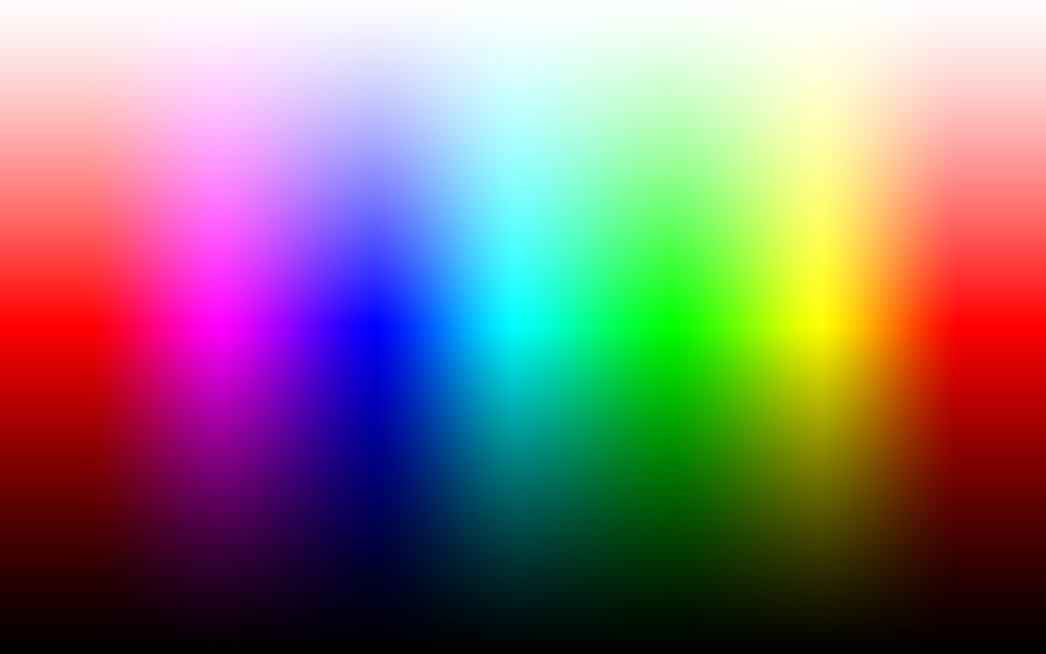
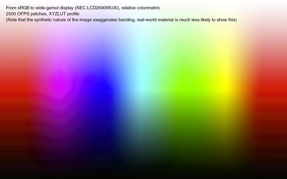
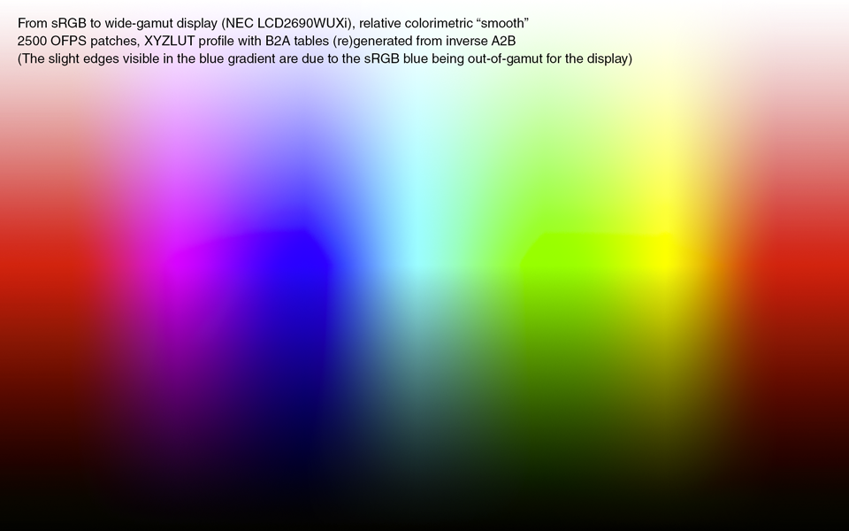
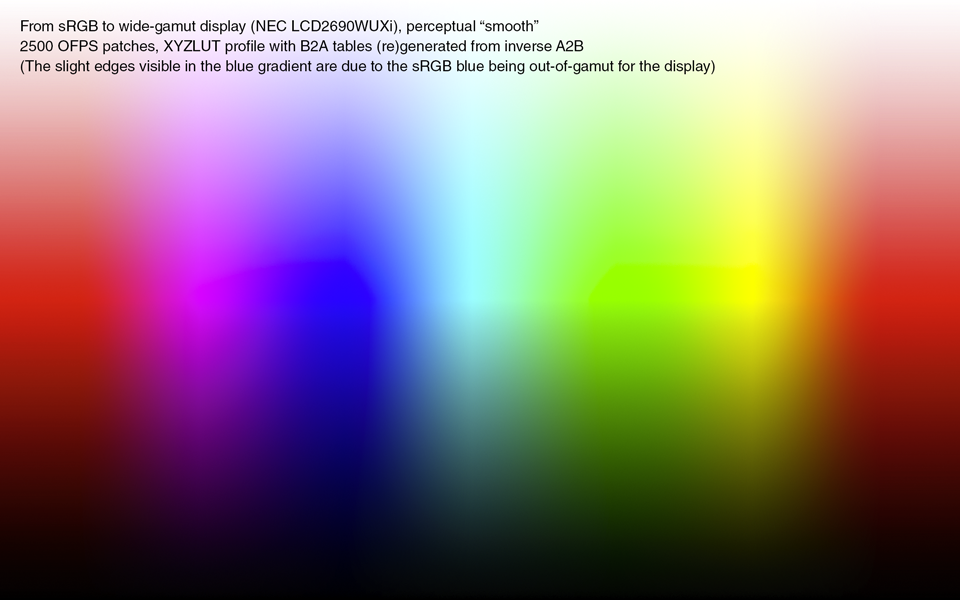
Calibrating / profiling
If you are unclear about the difference between calibration and profiling (also called characterization), see “Calibration vs. Characterization” in the ArgyllCMS documentation.
Please let the screen stabilize for at least half an hour after powering it up before doing any measurements or assessing its color properties. The screen can be used normally with other applications during that time.
After you have set your options, click on the button at the bottom to start the actual calibration/profiling process. The main window will hide during measurements, and should pop up again after they are completed (or after an error). You can always cancel out of running measurements using the “Cancel” button in the progress dialog, or by pressing ESC or Q. Viewing the informational log window (from the “Tools” menu) after measurements will give you access to the raw output of the ArgyllCMS commandline tools and other verbose information.
Adjusting a display before calibration
If you clicked “Calibrate” or “Calibrate & profile” and have not turned off “Interactive display adjustment”, you will be presented with the interactive display adjustment window which contains several options to help you bring a display's characteristics closer to the chosen target values. Depending on whether you have a “Refresh”- or LCD-type display, I will try to give some recommendations here which options to adjust, and which to skip.
Adjusting a LCD display
For LCD displays, you will in most cases only want to adjust white point (if the screen has RGB gain or other whitepoint controls) and white level (with the white level also affecting the black level unless you have a local dimming LED model), as many LCDs lack the necessary “offset” controls to adjust the black point (and even if they happen to have them, they often change the overall color temperature, not only the black point). Also note that for most LCD screens, you should leave the “contrast” control at (factory) default.
- White point
- If your screen has RGB gain, colortemperature or other whitepoint controls, the first step should be adjusting the whitepoint. Note that you may also benefit from this adjustment if you have set the target whitepoint to “native”, as it will allow you to bring it closer to the daylight or blackbody locus, which can help the human visual system to better adapt to the whitepoint. Look at the bars shown during the measurements to adjust RGB gains and minimize the delta E to the target whitepoint.
- White level
- Continue with the white level adjustment. If you have set a target white level, you may reduce or increase the brightness of your screen (ideally using only the backlight) until the desired value is reached (i.e. the bar ends at the marked center position). If you haven't set a target, simply adjust the screen to a visually pleasing brightness that doesn't cause eye strain.
Adjusting a “Refresh”-type display like CRT or Plasma
- Black level
- On “Refresh”-type displays, this adjustment is usually done using the “brightness” control. You may reduce or increase the brightness of your screen until the desired black level is reached (i.e. the bar ends at the marked center position).
- White point
- The next step should be adjusting the whitepoint, using the display's RGB gain controls or other means of adjusting the whitepoint. Note that you may also benefit from this adjustment if you have set the target whitepoint to “native”, as it will allow you to bring it closer to the daylight or blackbody locus, which can help the human visual system to better adapt to the whitepoint. Look at the bars shown during the measurements to adjust RGB gains and minimize the delta E to the target whitepoint.
- White level
- Continue with the white level adjustment. On “Refresh”-type displays this is usually done using the “contrast” control. If you have set a target white level, you may reduce or increase contrast until the desired value is reached (i.e. the bar ends at the marked center position). If you haven't set a target, simply adjust the screen to a visually pleasing level that doesn't cause eye strain.
- Black point
- If your display has RGB offset controls, you can adjust the black point as well, in much the same way that you adjusted the whitepoint.
Finishing adjustments and starting calibration/characterization
After the adjustments, you can run a check on all the settings by choosing the last option from the left-hand menu to verify the achieved values. If adjusting one setting adversely affected another, you can then simply repeat the respective option as necessary until the target parameters are met.
Finally, select “Continue on to calibration/profiling” to start the non-interactive part. Depending on the instrument you're using you may want to get a coffee or two as the process can take a fair amount of time, especially if you selected a slow speed level. If you only wanted help to adjust the display and don't want/need calibration curves to be created, you can also choose to exit by closing the interactive display adjustment window, then disable interactive adjustment, set calibration tone curve to “As measured” and then select “Profile only” from the main window.
If you originally selected “Calibrate & profile” and fulfil the requirements for unattended calibration & profiling, the characterization measurements for the profiling process should start automatically after calibration is finished. Otherwise, you may be forced to take the instrument off the screen to do a sensor self-calibration before starting the profiling measurements.
Optimizing testcharts for improved profiling accuracy and efficiency
The easiest way to use an optimized testchart for profiling is to set the testchart to “Auto” and adjusting the patch amount slider to the desired number of test patches. Optimization will happen automatically as part of the profiling measurements (this will increase measurement and processing times by a certain degree).
Alternatively, if you want to do generate an optimized chart manually prior to a new profiling run, you could go about this in the following way:
- Have a previous display profile and select it under “Settings”.
- Select one of the pre-baked testcharts to use as base and bring up the testchart editor.
- Next to “Preconditioning profile” click on “current profile”. It should automatically select the previous profile you've chosen. Then place a check in the checkbox. Make sure adaptation is set to a high level (e.g. 100%)
- If desired, adjust the number of patches and make sure the iterative patches amount is not zero.
- Create the chart and save it. Click “yes” when asked to select the newly generated chart.
- Start the profiling measurements (e.g. click “calibrate & profile”).
Profile installation
When installing a profile after creating or updating it, a startup item to load its calibration curves automatically on login will be created (on Windows and Linux, Mac OS X does not need a loader). You may also prevent this loader from doing anything by removing the check in the “Load calibration curves on Login” checkbox in the profile installation dialog, and in case you are using Windows 7 or later, you may let the operating system handle calibration loading instead (note that the Windows internal calibration loader does not offer the same high precision as the DisplayCAL profile loader, due to wrong scaling and 8-bit quantization).
Profile loader (Windows)
Under Windows, the profile loader will stay in the taskbar tray and keep the calibration loaded (unless started with the --oneshot argument, which will make the loader exit after loading calibration). In addition, the profile loader is madVR-aware and will disable calibration loading if it detects e.g. madTPG or madVR being used by a video player. You can double-click the profile loader system tray icon to instantly re-apply the currently selected calibration state (see below). A single click will show a popup with currently associated profiles and calibration information.
A right-click menu allows you to set the desired calibration state and a few other options:
- Load calibration from current display device profile(s). Selecting this (re)loads the calibration instantly, and also sets the desired calibration state (see “Preserve calibration state” below).
- Reset video card gamma table. Selecting this resets the video card gamma tables instantly, and also sets the desired calibration state (see “Preserve calibration state” below).
- Load calibration on login & preserve calibration state. This periodically checks if the video card gamma tables match the desired calibration state. It may take up to three seconds until the selected calibration state is automatically re-applied.
- Fix profile associations automatically when only one display is active in a multi-display setup. This is a work-around for applications (and Windows itself) querying the display profile in a way that does not take into account the active display, which can lead to a wrong profile being used. A pre-requisite for this working correctly is that the profile loader has to be running before you switch from a multi-display to a single-display configuration in Windows, and the profile associations have to be correct at this point. Note that quitting the profile loader will restore profile associations to what they were (honoring any changes to profile associations during its runtime). Also note that profile associations cannot be fixed (and the respective option will be disabled) in display configurations with three or more displays where some of them are deactivated.
- Show notifications when detecting a 3rd party calibration/profiling software or a user-defined exception (see below).
- Bitdepth. Some graphics drivers may internally quantize the video card gamma table values to a lower bitdepth than the nominal 16 bits per channel that are encoded in the video card gamma table tag of DisplayCAL-generated profiles. If this quantization is done using integer truncating instead of rounding, this may pronounce banding. In that case, you can let the profile loader quantize to the target bitdepth by using rounding, which may produce a smoother result.
- Exceptions. You can override the global profile loader state on a per application basis.
- Profile associations. Brings up a dialog where you can associate profiles to your display devices.
- Open Windows display settings.
Creating 3D LUTs
You can create display correction RGB-in/RGB-out 3D LUTs (for use in video playback or editing applications/devices that don't have ICC support) as part of the profiling process.
3D LUT settings
- Create 3D LUT after profiling
- Normally after profiling, you'll be given the option to install the profile to make it available for ICC color managed applications. If this box is checked, you'll have the option to generate a 3D LUT (with the chosen settings) instead, and the 3D LUT settings will also be stored inside the profile, so that they can be easily restored by selecting the profile under “Settings” if needed. If this box is unchecked, you can create a 3D LUT from an existing profile.
- Source colorspace/source profile
- This sets the source colorspace for the 3D LUT, which is normally a video standard space like defined by Rec. 709 or Rec. 2020.
- Tone curve
- This allows to set a predefined or custom tone response curve for the 3D LUT. Predefined settings are Rec. 1886 (input offset), Gamma 2.2 (output offset, pure power), SMPTE 2084 hard clip, SMPTE 2084 with roll-off (BT.2390-3) and Hybrid Log-Gamma (HLG).
Tone curve parameters
- “Absolute” vs. “Relative” gamma (not available for SMPTE 2084) To accomodate a non-zero black level of a real display, the tone response curve needs to be offset and scaled accordingly.
“Absolute” gamma results in an actual output at 50% input which doesn't match that of an idealized power curve (unless the black level is zero).
“Relative” gamma results in an actual output at 50% input which matches that of an idealized power curve. - Black output offset To accomodate a non-zero black level of a real display, the tone response curve needs to be offset and scaled accordingly. A black output offset of 0% (= all input offset) scales and offsets the input values (this matches BT.1886), while an offset of 100% scales and offsets the output values (this matches the overall curve shape of a pure power curve). A split between input and output offset is also possible.
- Target peak luminance (only available for SMPTE 2084) This allows you to adjust the clipping point (when not using roll-off) or roll-off to the desired target peak luminance. Note that you shouldn't necessarily enter your actual display peak white luminance here: For example, if you are using a display capable of 120 cd/m2, multiply with a factor between 3 to 5, i.e. enter 360 to 600 cd/m². The rule of thumb is to use a larger factor the lower your actual display peak luminance is (a dim projector may need a factor around 10), and a smaller factor (or none for an actual HDR display with at least 540 cd/m² capability) the higher it is.
- Preserve luminance/saturation (only available for SMPTE 2084 when advanced options are enabled in the “Options” menu) Can be used to set a split between preserving luminance vs saturation in rolled-off (or clipped) highlights. The default value of 50% provides a good balance between luminance and saturation. Note that setting a value above 50% may loose detail in very bright and saturated hues unless hue preservation is decreased in accordance (see below).
- Preserve hue (only available for SMPTE 2084 when advanced options are enabled in the “Options” menu) The default value of 50% allows certain very bright and saturated hues (red-orange/orange/amber) that have been subject to roll-off or clipping to gradually shift towards a more yellowish hue, better maintaining saturation and detail (selective hue shift). A value of 100% fully maintains the hue in rolled-off (or clipped) highlights.
- Mastering display black and peak luminance (only available for SMPTE 2084 roll-off when advanced options are enabled in the “Options” menu) HDR video content may not have been mastered on a display capable of showing the full range of HDR luminance levels, and so (optionally) altering the roll-off and specifying clipping points may be desirable to make better use of a target display's luminance capabilities.
A way to do this is to specify the mastering display black and peak luminance levels. Note that setting unsuitable values for a given video content may clip visually relevant information and introduce artifacts like banding, and therefore you should leave the mastering display black and peak luminance at their default values of 0 cd/m² and 10000 cd/m², respectively, if they cannot be reasonably assumed.
When mastering display peak luminance is set to a value below 10000 cd/m², you can choose whether the roll-off should be adjusted (more luminance, but potentially reduced detail near the peak) or not (less luminance, but potentially more detail near the peak). - Ambient luminance (only available for Hybrid Log-Gamma when advanced options are enabled in the “Options” menu) The default HLG system gamma of 1.2 (for a display with peak nominal luminance of 1000 cd/m² in a reference environment with 5 cd/m² ambient luminance) should be adjusted in non reference viewing environments. This is achieved by taking into account the ambient luminance (as per BT.2390-3).
- Content colorspace (only available for SMPTE 2084 roll-off when advanced options are enabled in the “Options” menu) HDR video content may not encode the full source gamut, and so compressing the actual encoded gamut (instead of the full source gamut) into the display gamut may be desirable. Note that there is usually no need to change this from the default (DCI P3), and that this setting has most impact on non-colorimetric rendering intents.
- HDR processing (convert HDR to SDR or pass through HDR) (only available for SMPTE 2084 when the 3D LUT format is set to madVR) Whether the 3D LUT will tell madVR to switch the display to HDR mode or not (HDR mode 3D LUTs will need to be set in the “process HDR content by an external 3D LUT” slot, HDR to SDR mode 3D LUTs in the “convert HDR content to SDR by using an external 3D LUT” slot in madVR's HDR options). Note that you need to have profiled the display in the respective mode (SDR or HDR) as well, and that DisplayCAL currently cannot switch a display into HDR mode.
- “Absolute” vs. “Relative” gamma (not available for SMPTE 2084) To accomodate a non-zero black level of a real display, the tone response curve needs to be offset and scaled accordingly.
- Apply calibration (vcgt) (only visible if “Show advanced options” in the “Options” menu is enabled)
- Apply the profile's 1D LUT calibration (if any) to the 3D LUT. Normally, this should always be enabled if the profile contains a non-linear 1D LUT calibration, otherwise you have to make sure the 1D calibration is loaded whenever the 3D LUT is used.
- Gamut mapping mode (only visible if “Show advanced options” in the “Options” menu is enabled)
- The default gamut mapping mode is “Inverse device to PCS” and gives the most accurate results. In case a profile with high enough PCS-to-device table resolution is used, the option “PCS-to-device” is selectable as well, which allows for quicker generation of a 3D LUT, but is somewhat less accurate.
- Rendering intent
-
- “Absolute colorimetric” is intended to reproduce colors exactly. Out of gamut colors will be clipped to the closest possible match. The destination whitepoint will be altered to match the source whitepoint if possible, which may get clipped if it is out of gamut.
- “Absolute appearance” maps colors from source to destination, trying to match the appearance of colors as closely as possible, but may not exactly map the whitepoint. Out of gamut colors will be clipped to the closest possible match.
- “Absolute colorimetric with white point scaling” behaves almost exactly like “Absolute colorimetric”, but will scale the source colorspace down to make sure the source whitepoint isn't clipped.
- “Luminance matched appearance” linearly compresses or expands the luminance axis from white to black to match the source to the destination space, while not otherwise altering the gamut, clipping any out of gamut colors to the closest match. The destination whitepoint is not altered to match the source whitepoint.
- “Perceptual” uses three-dimensional compression to make the source gamut fit within the destination gamut. As much as possible, clipping is avoided, hues and the overall appearance is maintained. The destination whitepoint is not altered to match the source whitepoint. This intent is useful if the destination gamut is smaller than the source gamut.
- “Perceptual appearance” uses three-dimensional compression to make the source gamut fit within the destination gamut. As much as possible, clipping is avoided, hues and the overall appearance is maintained. The destination whitepoint is altered to match the source whitepoint. This intent is useful if the destination gamut is smaller than the source gamut.
- “Luminance preserving perceptual” (ArgyllCMS 1.8.3+) uses compression to make the source gamut fit within the destination gamut, but very heavily weights the preservation of the luminance value of the source, which will compromise the preservation of saturation. No contrast enhancement is used if the dynamic range is reduced. This intent may be of use where preserving the tonal distinctions in images is more important than maintaining overall colorfulness or contrast.
- “Preserve saturation” uses three-dimensional compression and expansion to try and make the source gamut match the destination gamut, and also favours higher saturation over hue or lightness preservation. The destination whitepoint is not altered to match the source whitepoint.
- “Relative colorimetric” is intended to reproduce colors exactly, but relative to the destination whitepoint which will not be altered to match the source whitepoint. Out of gamut colors will be clipped to the closest possible match. This intent is useful if you have calibrated a display to a custom whitepoint that you want to keep.
- “Saturation” uses the same basic gamut mapping as “Preserve saturation”, but increases saturation slightly in highly saturated areas of the gamut.
- 3D LUT file format
- Sets the output format for the 3D LUT. Currently supported are Autodesk/Kodak (
.3dl), Iridas (.cube), eeColor (.txt), madVR (.3dlut), Pandora (.mga), Portable Network Graphic (.png), ReShade (.png,.fx) and Sony Imageworks (.spi3d). Note that an ICC device link profile (the ICC equivalent of an RGB-in/RGB-out 3D LUT) is always created as well. - Input/output encoding
- Some 3D LUT formats allow you to set the input/output encoding. Note that in most cases, sensible defaults will be chosen depending on selected 3D LUT format, but may be application- or workflow-specific.
- Input/output bit depth
- Some 3D LUT formats allow you to set the input/output bit depth. Note that in most cases, sensible defaults will be chosen depending on selected 3D LUT format, but may be application- or workflow-specific.
Installing 3D LUTs
Depending on the 3D LUT file format, installing or saving the 3D LUT to a specific location may be required before it can be used. You will be asked to install or save the 3D LUT directly after it was created. If you need to install or save the 3D LUT again at a later point, switch to the “3D LUT” tab and click the small “Install 3D LUT” button next to the “Settings” dropdown (the same button that installs display profiles when on the “Display & instrument” tab and a directly connected, desktop-accessible display is selected).
Installing 3D LUTs for the ReShade injector
First, you need to download the latest version of ReShade and extract the ZIP file. This should result in a folder “ReShade <version>”. Then, install the 3D LUT from within DisplayCAL to the “ReShade <version>” folder (select the folder when prompted). This will activate the 3D LUT for all applications/games that you're going to use ReShade with, which you can configure using the “ReShade Assistant” application that should come with ReShade (refer to the instructions available on the ReShade website on how to configure ReShade). The default toggle key to turn the 3D LUT on and off is the HOME key. You can change this key or disable the 3D LUT altogether by editing ColorLookUpTable.fx (with a text editor) inside the “ReShade <version>” folder where you installed the 3D LUT. To remove the 3D LUT from ReShade completely, delete ColorLookUpTable.png and ColorLookUpTable.fx in the ReShade folder, as well as edit ReShade.fx and remove the line #include "ColorLookupTable.fx" near the end.
Verification / measurement report
You can do verification measurements to assess the display chain's (display profile - video card and the calibration curves in its gamma table - monitor) fit to the measured data, or to find out about the soft proofing capabilities of the display chain. You can also do a profile or device link (3D LUT) self check without having to take any further measurements by holding the “alt” key on your keyboard.
To check the fit to the measurement data, you have to select a CGATS[1] testchart file containing device values (RGB). The measured values are then compared to the values obtained by feeding the device RGB numbers through the display profile (measured vs expected values). The default verification chart contains 26 patches and can be used, for example, to check if a display needs to be re-profiled. If a RGB testchart with gray patches (R=G=B) is measured, like the default and extended verification charts, you also have the option to evaluate the graybalance through the calibration only, by placing a check in the corresponding box on the report.
To perform a check on the soft proofing capabilities, you have to provide a CGATS reference file containing XYZ or L*a*b* data, or a combination of simulation profile and testchart file, which will be fed through the display profile to lookup corresponding device (RGB) values, and then be sent to the display and measured. Afterwards, the measured values are compared to the original XYZ or L*a*b* values, which can give a hint how suitable (or unsuitable) the display is for softproofing to the colorspace indicated by the reference.
The profile that is to be evaluated can be chosen freely. You can select it in DisplayCAL's main window under “settings”. The report files generated after the verification measurements are plain HTML with some embedded JavaScript, and are fully self-contained. They also contain the reference and measurement data, which consists of device RGB numbers, original measured XYZ values, and D50-adapted L*a*b* values computed from the XYZ numbers, and which can be examined as plain text directly from the report at the click of a button.
HowTo—Common scenarios
Select the profile you want to evaluate under “Settings” (for evaluating 3D LUTs and DeviceLink profiles, this setting has significance for a Rec. 1886 or custom gamma tone response curve, because they depend on the black level).
There are two sets of default verification charts in different sizes, one for general use and one for Rec. 709 video. The “small” and “extended” versions can be used for a quick to moderate check to see if a display should be re-profiled, or if the used profile/3D LUT is any good to begin with. The “large” and “xl” versions can be used for a more thorough check. Also, you can create your own customized verification charts with the testchart editor.
Checking the accuracy of a display profile (evaluating how well the profile characterizes the display)
In this case, you want to use a testchart with RGB device values and no simulation profile. Select a suitable file under “testchart or reference” and disable “simulation profile”. Other settings that do not apply in this case will be grayed out.
Checking how well a display can simulate another colorspace (evaluating softproofing capabilities, 3D LUTs, DeviceLink profiles, or native display performance)
There are two ways of doing this:
- Use a reference file with XYZ or L*a*b* aim values,
- or use a combination of testchart with RGB or CMYK device values and an RGB or CMYK simulation profile (for an RGB testchart, it will only allow you to use an RGB simulation profile and vice versa, and equally a CMYK testchart needs to be used with a CMYK simulation profile)
Then, you have a few options that influence the simulation.
- Whitepoint simulation. If you are using a reference file that contains device white (100% RGB or 0% CMYK), or if you use a combination of testchart and simulation profile, you can choose if you want whitepoint simulation of the reference or simulation profile, and if so, if you want the whitepoint simulated relative to the display profile whitepoint. To explain the latter option: Let's assume a reference has a whitepoint that is slightly blueish (compared to D50), and a display profile has a whitepoint that is more blueish (compared to D50). If you do not choose to simulate the reference white relative to the display profile whitepoint, and the display profile's gamut is large and accurate enough to accomodate the reference white, then that is exactly what you will get. Depending on the adaptation state of your eyes though, it may be reasonable to assume that you are to a large extent adapted to the display profile whitepoint (assuming it is valid for the device), and the simulated whitepoint will look a little yellowish compared to the display profile whitepoint. In this case, choosing to simulate the whitepoint relative to that of the display profile may give you a better visual match e.g. in a softproofing scenario where you compare to a hardcopy proof under a certain illuminant, that is close to but not quite D50, and the display whitepoint has been matched to that illuminant. It will “add” the simulated whitepoint “on top” of the display profile whitepoint, so in our example the simulated whitepoint will be even more blueish than that of the display profile alone.
-
Using the simulation profile as display profile will override the profile set under “Settings”. Whitepoint simulation does not apply here because color management will not be used and the display device is expected to be in the state described by the simulation profile. This may be accomplished in several ways, for example the display may be calibrated internally or externally, by a 3D LUT or device link profile. If this setting is enabled, a few other options will be available:
- Enable 3D LUT (if using the madVR display device/madTPG under Windows, or a Prisma video processor). This allows you to check how well the 3D LUT transforms the simulation colorspace to the display colorspace. Note this setting can not be used together with a DeviceLink profile.
- DeviceLink profile. This allows you to check how well the DeviceLink transforms the simulation colorspace to the display colorspace. Note this setting can not be used together with the “Enable 3D LUT” setting.
-
Tone response curve. If you are evaluating a 3D LUT or DeviceLink profile, choose the same settings here as during 3D LUT/DeviceLink creation (and also make sure the same display profile is set, because it is used to map the blackpoint).
To check a display that does not have an associated profile (e.g. “Untethered”), set the verification tone curve to “Unmodified”. In case you want to verify against a different tone response curve instead, you need to create a synthetic profile for this purpose (“Tools” menu).
How were the nominal and recommended aim values chosen?
The nominal tolerances, with the whitepoint, average, maximum and gray balance Delta E CIE 1976 aim values stemming from UGRA/Fogra Media Wedge and UDACT, are pretty generous, so I've included somewhat stricter “recommended” numbers which I've chosen more or less arbitrarily to provide a bit “extra safety margin”.
For reports generated from reference files that contain CMYK numbers in addition to L*a*b* or XYZ values, you can also select the official Fogra Media Wedge V3 or IDEAlliance Control Strip aim values for paper white, CMYK solids and CMY grey, if the chart contains the right CMYK combinations.
How are the results of the profile verification report to be interpreted?
This depends on the chart that was measured. The explanation in the first paragraph sums it up pretty well: If you have calibrated and profiled your display, and want to check how well the profile fits a set of measurements (profile accuracy), or if you want to know if your display has drifted and needs to be re-calibrated/re-profiled, you select a chart containing RGB numbers for the verification. Note that directly after profiling, accuracy can be expected to be high if the profile characterizes the display well, which will usually be the case if the display behaviour is not very non-linear, in which case creating a LUT profile instead of a “Curves + matrix” one, or increasing the number of measured patches for LUT profiles, can help.
If you want to know how well your profile can simulate another colorspace (softproofing), select a reference file containing L*a*b* or XYZ values, like one of the Fogra Media Wedge subsets, or a combination of a simulation profile and testchart. Be warned though, only wide-gamut displays will handle a larger offset printing colorspace like FOGRA39 or similar well enough.
In both cases, you should check that atleast the nominal tolerances are not exceeded. For a bit “extra safety margin”, look at the recommended values instead.
Note that both tests are “closed-loop” and will not tell you an “absolute” truth in terms of “color quality” or “color accuracy” as they may not show if your instrument is faulty/measures wrong (a profile created from repeatable wrong measurements will usually still verify well against other wrong measurements from the same instrument if they don't fluctuate too much) or does not cope with your display well (which is especially true for colorimeters and wide-gamut screens, as such combinations need a correction in hardware or software to obtain accurate results), or if colors on your screen match an actual colored object next to it (like a print). It is perfectly possible to obtain good verification results but the actual visual performance being sub-par. It is always wise to combine such measurements with a test of the actual visual appearance via a “known good” reference, like a print or proof (although it should not be forgotten that those also have tolerances, and illumination also plays a big role when assessing visual results). Keep all that in mind when admiring (or pulling your hair out over) verification results :)
How are profiles evaluated against the measured values?
Different softwares use different methods (which are not always disclosed in detail) to compare and evaluate measurements. This section aims to give interested users a better insight how DisplayCAL's profile verification feature works “under the hood”.
How is a testchart or reference file used?
There are currently two slightly different paths depending if a testchart or reference file is used for the verification measurements, as outlined above. In both cases, Argyll's xicclu utility is run behind the scenes and the values of the testchart or reference file are fed relative colorimetrically (if no whitepoint simualtion is used) or absolute colorimetrically (if whitepoint simulation is used) through the profile that is tested to obtain corresponding L*a*b* (in the case of RGB testcharts) or device RGB numbers (in the case of XYZ or L*a*b* reference files or a combination of simulation profile and testchart). If a combination of simulation profile and testchart is used as reference, the reference L*a*b* values are calculated by feeding the device numbers from the testchart through the simulation profile absolute colorimetrically if whitepoint simulation is enabled (which will be the default if the simulation profile is a printer profile) and relative colorimetrically if whitepoint simulation is disabled (which will be the default if the simulation profile is a display profile, like most RGB working spaces). Then, the original RGB values from the testchart, or the looked up RGB values for a reference are sent to the display through the calibration curves of the profile that is going to be evaluated. A reference white of D50 (ICC default) and complete chromatic adaption of the viewer to the display's whitepoint is assumed if “simulate whitepoint relative to display profile whitepoint” is used, so the measured XYZ values are adapted to D50 (with the measured whitepoint as source reference white) using the Bradford transform (see Chromatic Adaption on Bruce Lindbloom's website for the formula and matrix that is used by DisplayCAL) or with the adaption matrix from the profile in the case of profiles with 'chad' chromatic adaption tag, and converted to L*a*b*. The L*a*b* values are then compared by the generated dynamic report, with user-selectable critera and ΔE (delta E) formula.
How is the assumed vs. measured whitepoint ΔE calculated?
In a report, the correlated color temperature and assumed target whitepoint, as well as the whitepoint ΔE, do warrant some further explanations: The whitepoint ΔE is calculated as difference between the measured whitepoint's and the assumed target whitepoint's normalized XYZ values, which are first converted to L*a*b*. The assumed target whitepoint color temperature shown is simply the rounded correlated color temparature (100K threshold) calculated from the measured XYZ values. The XYZ values for the assumed target whitepoint are obtained by calculating the chromaticity (xy) coordinates of a CIE D (daylight) or blackbody illuminant of that color temperature and converting them to XYZ. You can find all the used formulas on Bruce Lindbloom's website and on Wikipedia.
How is the gray balance “range” evaluated?
The gray balance “range” uses a combined delta a/delta b absolute deviation (e.g. if max delta a = -0.5 and max delta b = 0.7, the range is 1.2). Because results in the extreme darks can be problematic due to lack of instrument accuracy and other effects like a black point which has a different chromaticity than the whitepoint, the gray balance check in DisplayCAL only takes into account gray patches with a minimum measured luminance of 1% (i.e. if the white luminance = 120 cd/m², then only patches with at least 1.2 cd/m² will be taken into account).
What does the “Evaluate gray balance through calibration only” checkbox on a report actually do?
It sets the nominal (target) L* value to the measured L* value and a*=b*=0, so the profile is effectively ignored and only the calibration (if any) will influence the results of the gray balance checks. Note that this option will not make a difference for a “Single curve + matrix” profile, as the single curve effectively already achieves a similar thing (the L* values can be different, but they are ignored for the gray balance checks and only influence the overall result).
What do the “Use absolute values” and “Use display profile whitepoint as reference white” checkboxes on a report do?
If you enable “Use absolute values” on a report, the chromatic adaptation to D50 is undone (but the refrence white for the XYZ to L*a*b* conversion stays D50). This mode is useful when checking softproofing results using a CMYK simulation profile, and will be automatically enabled if you used whitepoint simulation during verification setup without enabling whitepoint simulation relative to the profile whitepoint (true absolute colorimetric mode). If you enable “Use display profile whitepoint as reference white”, then the reference white used for the XYZ to L*a*b* conversion will be that of the display profile, which is useful when verifying video calibrations where the target is usually some standard color space like Rec. 709 with a D65 equivalent whitepoint.
Special functionality
Remote measurements and profiling
When using ArgyllCMS 1.4.0 and newer, remote measurements on a device not directly connected to the machine that is running DisplayCAL is possible (e.g. a smartphone or tablet). The remote device needs to be able to run a web browser (Firefox recommended), and the local machine running DisplayCAL may need firewall rules added or altered to allow incoming connections. To set up remote profiling, select “Web @ localhost” from the display device dropdown menu, then choose the desired action (e.g. “Profile only”). When the message “Webserver waiting at http://<IP>:<Port>” appears, open the shown address in the remote browser and attach the measurement device.
NOTE: If you use this method of displaying test patches, there is no access to the display video LUT[7]s and hardware calibration is not possible. The colors will be displayed with 8 bit per component precision, and any screen-saver or power-saver will not be automatically disabled. You will also be at the mercy of any color management applied by the web browser, and may have to carefully review and configure such color management.
Note: Close the web browser window or tab after each run, otherwise reconnection may fail upon further runs.
madVR test pattern generator
DisplayCAL supports the madVR test pattern generator (madTPG) and madVR 3D LUT formats since version 1.5.2.5 when used together with ArgyllCMS 1.6.0 or newer.
Resolve (10.1+) as pattern generator
Since version 2.5, DisplayCAL can use Resolve (10.1+) as pattern generator. Select the “Resolve” entry from the display devices dropdown in DisplayCAL and in Resolve itself choose “Monitor calibration”, “CalMAN” in the “Color” menu.
Untethered display measurements
Please note that the untethered mode should generally only be used if you've exhausted all other options.
Untethered mode is another option to measure and profile a remote display that is not connected via standard means (calibration is not supported). To use untethered mode, the testchart that should be used needs to be optimized, then exported as image files (via the testchart editor) and those image files need to be displayed on the device that should be measured, in successive order. The procedure is as follows:
- Select the desired testchart, then open the testchart editor.
- Select “Maximize lightness difference” from the sorting options dropdown, click “Apply”, then export the testchart.
- Burn the images to a DVD, copy them on an USB stick or use any other available means to get them to display onto the device that should be measured.
- In DisplayCAL's display dropdown, select “Untethered” (the last option).
- Show the first image on the remote display, and attach the instrument. Then select “Profile only”.
Measurements will commence, and changes in the displayed image should be automatically detected if “auto” mode is enabled. Use whatever means available to you to cycle through the images from first to last, carefully monitoring the measurement process and only changing to the next image if the current one has been successfully measured (as will be shown in the untethered measurement window). Note that untethered mode will be (atleast) twice as slow as normal display measurements.
Non-UI functionality
There is a bit of functionality that is not available via the UI and needs to be run from a command prompt or ternminal. Use of this functionality currently requires running from source.
- Change display profile and calibration whitepoint
-
Note that this reduces the profile gamut and accuracy.
From source:
python util/change_display_profile_cal_whitepoint.py \

  [-t temp | -T temp | -w x,y] [--cal-only] [inprofile] outfilename
-t temp- Use daylight color temperature
tempas whitepoint target. -T temp- Use blackbody color temperature
tempas whitepoint target. -w x,y- Use x,y chromaticity as whitepoint target.
--cal-only(optional)- Only alter the calibration embedded in the profile, not the profile itself.
inprofile(optional)- Use profile
inprofileinstead of the current display profile. outfilename- Output profile filename. The changed profile will be written to this file.
- Enable/disable Windows 7 and later calibration loading
-
Note that Windows calibration loading is of lower quality than using ArgyllCMS because Windows always quantizes the calibration to 8 bit and scales it wrongly. This is not the case when using the DisplayCAL calibration loader which uses ArgyllCMS.
From source:
python -c "import sys; from DisplayCAL import util_win; \

  util_win.calibration_management_isenabled() or \

  util_win.enable_calibration_management() \

  if '--os' in sys.argv[1:] else \

  not util_win.calibration_management_isenabled() or \

  util_win.disable_calibration_management();" [--os]
The
--osoption determines wether Windows calibration loading functionality should be enbaled or disabled.
Scripting
DisplayCAL supports scripting locally and over the network (the latter must be explicitly enabled by setting app.allow_network_clients = 1 in DisplayCAL.ini) via sockets. DisplayCAL must be already running on the target machine for this to work. Below is an example connecting to a running instance on the default port 15411 and starting calibration measurements (the port is configurable in DisplayCAL.ini as app.port, although if the desired port is not available an unused one will be chosen automatically. You can read the actual used port from the file DisplayCAL.lock in the configuration file folder of DisplayCAL while it is running). The example is written in Python and deals with some of the intricacies of sockets as well.
#!/usr/bin/env python2

import socket

class DCGScriptingClientSocket(socket.socket):

	def __enter__(self):
		return self

	def __exit__(self, etype, value, tb):
		# Disconnect
		try:
			# Will fail if the socket isn't connected, i.e. if there was an
			# error during the call to connect()
			self.shutdown(socket.SHUT_RDWR)
		except socket.error:
			pass
		self.close()

	def __init__(self):
		socket.socket.__init__(self)
		self.recv_buffer = ''

	def get_single_response(self):
		# Buffer received data until EOT (response end marker) and return
		# single response (additional data will still be in the buffer)
		while not '\4' in self.recv_buffer:
			incoming = self.recv(4096)
			if incoming == '':
				raise socket.error("Connection broken")
			self.recv_buffer += incoming
		end = self.recv_buffer.find('\4')
		single_response = self.recv_buffer[:end]
		self.recv_buffer = self.recv_buffer[end + 1:]
		return single_response

	def send_and_check(self, command, expected_response="ok"):
		""" Send command, get & check response """
		self.send_command(command)
		single_response = self.get_single_response()
		if single_response != expected_response:
			# Check application state. If a modal dialog is displayed, choose
			# the OK option. Note that this is just an example and normally you
			# should be very careful with this, as it could mean confirming a
			# potentially destructive operation (e.g. discarding current
			# settings, overwriting existing files etc).
			self.send_command('getstate')
			state = self.get_single_response()
			if 'Dialog' in state.split()[0]:
				self.send_command('ok')
				if self.get_single_response() == expected_response:
					return
			raise RuntimeError('%r got unexpected response: %r != %r' %
							   (command, single_response, expected_response))

	def send_command(self, command):
		# Automatically append newline (command end marker)
		self.sendall(command + '\n')

# Generate a list of commands we want to execute in order
commands = []

# Load “Laptop” preset
commands.append('load presets/laptop.icc')

# Setup calibration & profiling measurements
commands.append('calibrate-profile')

# Start actual measurements
commands.append('measure')

# Create socket & send commands
with DCGScriptingClientSocket() as client:
	client.settimeout(3)  # Set a timeout of 3 seconds

	# Open connection
	client.connect(('127.0.0.1', 15411))  # Default port

	for command in commands:
		client.send_and_check(command)
Each command needs to be terminated with a newline character (after any arguments the command may accept). Note that data sent must be UTF-8 encoded, and if arguments contain spaces they should be encased in double or single quotes. You should check the response for each command sent (the response end marker is ASCII 0x4 EOT, and the default response format is a plain text format, but JSON and XML are also available). The common return values for commands are either ok in case the command was understood (note that this does not indicate if the command finished processing), busy or blocked in case the command was ignored because another operation was running or a modal dialog blocks the UI, failed in case the command or an argument could not be processed successfully, forbidden in case the command was not allowed (this may be a temporary condition depending on the circumstances, e.g. when trying to interact with an UI element that is currently disabled), invalid in case the command (or one of its arguments) was invalid, or error followed by an error message in case of an unhandled exception. Other return values are possible depending on the command. All values returned are UTF-8 encoded. If the return value is blocked (e.g. because a modal dialog is displayed) you should check the application state with the getstate command to determine the further course of action.
List of supported commands
Below is a list of the currently supported commands (the list contains all valid commands for the main application, the standalone tools will typically just support a smaller subset. You can use the “DisplayCAL Scripting Client” standalone tool to learn about and experiment with commands). Note that filename arguments must refer to files present on the target machine running DisplayCAL.
3DLUT-maker [create filename]- Show 3D LUT creation tab, or create 3D LUT
filename. abort- Try to abort a currently running operation.
activate [window ID | name | label]- Activate window
windowor the main application window (bring it to the front). If it is minimized, restore it. alt | cancel | ok [filename]- If a modal dialog is shown, call the default action (ok), the alternate action (if applicable), or cancel it. If a file dialog is shown, using
ok filenamechooses that file. calibrate- Setup calibration measurements (note that this won't give a choice whether to create a fast curves + matrix profile as well, if you want that use
interact mainframe calibrate_btninstead). For non-virtual displays as well as pattern generators (except madVR), call themeasurecommand afterwards to commence measurements. calibrate-profile- Setup calibration & profiling measurements. For non-virtual displays as well as pattern generators (except madVR), call the
measurecommand afterwards to commence measurements. close [window ID | name | label]- Close window
windowor the current active window (if the window is the main window, this quits the application). Note that this tries to abort any running operations first, so you may want to check application state via thegetstatecommand. create-colorimeter-correction- Create colorimeter correction.
create-profile [filename]- Create profile from existing measurements (profile or measurement file).
curve-viewer [filename]- Show curves, optionally loading
filename. Relative paths are possible e.g. for presets:curve-viewer presets/photo.icc DisplayCAL [filename]- Bring the main window to the front. If it is minimized, restore it. Optionally, load
filename. enable-spyder2- Enable the spyder 2.
getactivewindow- Get the current active window. The returned format is
classnameIDnamelabelstate.stateis eitherenabledordisabled. getcellvalues [window ID | name | label] <grid ID | name | label>- Get cell values from grid
gridof windowwindowor the current active window. getappname- Get the name of the application you're connected to.
getcfg [option]- Get configuration
option, or whole configuration (key-value pairs in INI format). getcommands- Get list of commands supported by this application.
getdefault <option>- Get default
option(key-value pair in INI format). getdefaults- Get all defaults (key-value pairs in INI format).
- Get available menus in the format
ID "label" state.stateis eitherenabledordisabled. - Get available menu items in the format
menuposition"menulabel"menuitemID"menuitemlabel"state[checkable][checked].stateis eitherenabledordisabled. getstate- Get application state. Return value will be either
idle,busy,dialogclassnameIDdialogname[dialoglabel]state"messagetext"[path "path"][buttons "buttonlabel"...]if a modal dialog is shown orblockedin case the UI is currently blocked. Most commands will not work if the UI is blocked—the only way to resolve the block is to non-programmatically interact with the actual UI elements of the application or closing it. Note that a state ofblockedshould normally only occur if an actual file dialog is shown. If using the scripting interface exclusively, this should never happen because it uses a replacement file dialog that supports the same actions as a real file dialog, but doesn't block. Also note that a return value ofblockedfor any of the other commands just means that a modal dialog is currently waiting to be interacted with, only ifgetstatealso returnsblockedyou cannot resolve the situation with scripting alone. getuielement [window ID | name | label] <element ID | name | label>getuielements [window ID | name | label]- Get a single UI element or a list of the visible UI elements of window
windowor the current active window. Each returned line represents an UI element and has the formatclassnameIDname["label"]state[checked][value "value"][items "item"...].classnameis the internal UI library class name. It can help you determine what type of UI element it is, and which interactions it supports.IDis a numeric identifier.nameis the name of the UI element."label"(if present) is a label which further helps in identifying the UI element. You can use the latter three with theinteractcommand.stateis eitherenabledordisabled.items "item"...(if present) is a list of items connected to the UI element (i.e. selection choices). getvalid- Get valid values for options that have constraints (key-value pairs in INI format). There are two sections,
rangesandvalues.rangesare the valid ranges for options that accept numeric values (note that integer options not covered byrangesare typically boolean types).valuesare the valid values for options that only accept certain values. Options not covered byrangesandvaluesare limited to their data type (you can't set a numeric option to a string and vice versa). getwindows- Get a list of visible windows. The returned format is a list of
classnameIDnamelabelstate.stateis eitherenabledordisabled. import-colorimeter-corrections [filename...]- Import colorimeter corrections.
install-profile [filename]- Install a profile.
interact [window ID | name | label] <element ID | name | label> [setvalue value]- Interact with the UI element
elementof windowwindowor the current active window, e.g. invoke a button or set a control to a value. - Invoke a menu item.
load <filename>- Load
filename. Relative paths are possible e.g. for presets:load presets/photo.icc measure- Start measurements (must be setup first!).
measure-uniformity- Measure screen uniformity.
measurement-report [filename]- If no filename given, show measurement report tab. Otherwise, setup measurement to create the HTML report
filename. For non-virtual displays as well as pattern generators (except madVR), call themeasurecommand afterwards to commence measurements. profile- Setup profiling measurements (note that this will always use the current calibration if applicable, if you want to use linear calibration instead call
load linear.calprior to callingprofile). For non-virtual displays as well as pattern generators (except madVR), call themeasurecommand afterwards to commence measurements. profile-info [filename]- Show profile information, optionally loading profile
filename. Relative paths are possible e.g. for presets:profile-info presets/photo.icc refresh- Update the GUI after configuration changes via
setcfgorrestore-defaults. report-calibrated- Report on calibrated display. For non-virtual displays as well as pattern generators (except madVR), call the
measurecommand afterwards to commence measurements. report-uncalibrated- Report on uncalibrated display. For non-virtual displays as well as pattern generators (except madVR), call the
measurecommand afterwards to commence measurements. restore-defaults [category...]- Restore defaults globally or just for
category. Callrefreshafter changing the configuration to update the GUI. setlanguage <languagecode>- Set language.
setcfg <option> <value>- Set configuration
optiontovalue. The special valuenullclears a configuration option. Callrefreshafter changing the configuration to update the GUI. Also seegetdefaultsandgetvalid. setresponseformat <format>- Set the format for responses. The default
plainis a text format that is easy to read, but not necessarily the best for parsing programmatically. The other possible formats arejson,json.pretty,xmlandxml.pretty. The*.prettyformats use newlines and indentation to make them easier to read. synthprofile [filename]- Show synthetic profile creation window, optionally loading profile
filename. testchart-editor [filename | create filename]- Show testchart editor window, optionally loading or creating testchart
filename. Relative paths are possible e.g. for loading a default testchart:testchart-editor ti1/d3-e4-s17-g49-m5-b5-f0.ti1 verify-calibration- Verify calibration. For non-virtual displays as well as pattern generators (except madVR), call the
measurecommand afterwards to commence measurements.
Interacting with UI elements
- Invoking a button:
interact [window] <button>e.g. show profile name placeholders information:interact mainframe profile_name_info_btn - Setting a value on a dropdown, text field, or slider:
interact [window] <element> setvalue "value"e.g. set calibration gamma to 2.4:interact mainframe trc_textctrl setvalue 2.4(note that for changing multiple options at once it is generally preferable to callsetcfg <option> <value>for each option you want to set followed by a singlerefreshinstead) - Setting a cell value on a grid:
interact [window] <grid> setvalue "row,col,value"e.g. while the testchart editor is shown, set the cell at the second column of the first row to 33:interact tcgen grid setvalue "0,1,33"
Caveats and limitations
There are a few things to be aware of when using commands that interact with the UI directly (i.e. activate, alt | cancel | ok, close, interact and invokemenu).
Referring to windows and UI elements: You can refer to windows and UI elements by their ID, name or label (you can find out about windows and UI elements with the getmenus/getmenuitems, getuielement/getuielements, and getwindows commands). If an object's ID is negative, it means that it has been automatically assigned at object creation time and is only valid during the lifetime of the object (i.e. for modal dialogs, only while the dialog is displayed). For this reason, using an object's name instead is easier, but names (aswell as non automatically assigned IDs) are not guaranteed to be unique, even for objects which share the same parent window (although most of the “important” controls as well as application windows will have unique names). Another possibility is to use an object's label, which while also not guaranteed to be unique, still has a fairly high likelihood of being unique for controls that share the same parent window, but has the drawback that it is localized (although you can ensure a specific UI language by calling setlanguage) and is subject to change when the localization is updated.
Sequential operations: Calling commands that interact with the UI in rapid succession may require the use of additional delays between sending commands to allow the GUI to react (so getstate will return the actual UI state after a specific command), although there is a default delay for commands that interact with the UI of atleast 55 ms. A good rule of thumb for sending commands is to use a “send command” → “read response” → “optionally wait a few extra ms” → “get application state (send getstate command)” → “read response” cycle.
Setting values: If setting a value on an UI element returns ok, this is not always an indication that the value was actually changed, but only that the attempt to set the value has not failed, i.e. the event handler of the element may still do error checking and change the value to something sane if it was not valid. If you want to make sure that the intended value is set, use getuielement on the affected element(s) and check the value (or even better, if you use JSON or XML response format, you can check the object property/element of the response instead which will reflect the object's current state and saves you one request). In general it is preferable to use interact <elementname> setvalue <value> only on dialogs, and in all other cases use a sequence of setcfg <option> <value> (repeat as necessary, optionally call load <filename> or restore-defaults first to minimize the amount of configuration options that you need to change) followed by a call to refresh to update the UI.
Also, not all controls may offer a comprehensive scripting interface. I'm open to suggestions though.
User data and configuration file locations
DisplayCAL uses the following folders for configuration, logfiles and storage (the storage directory is configurable). Note that if you have upgraded to DisplayCAL from dispcalGUI, that DisplayCAL will continue to use the existing dispcalGUI directories and configuration file names (so replace DisplayCAL with dispcalGUI in the lists below).
Configuration
- Linux: /home/Your Username/.config/DisplayCAL
- Mac OS X: /Users/Your Username/Library/Preferences/DisplayCAL
- Windows Vista and newer: C:\Users\Your Username\AppData\Roaming\DisplayCAL
- Windows XP: C:\Documents and Settings\Your Username\Application Data\DisplayCAL
Logs
- Linux: /home/Your Username/.local/share/DisplayCAL/logs
- Mac OS X:
/Users/Your Username/Library/Logs/DisplayCAL and
- Windows Vista and newer: C:\Users\Your Username\AppData\Roaming\DisplayCAL\logs
- Windows XP: C:\Documents and Settings\Your Username\Application Data\DisplayCAL\logs
Storage
- Linux: /home/Your Username/.local/share/DisplayCAL/storage
- Mac OS X: /Users/Your Username/Library/Application Support/DisplayCAL/storage
- Windows Vista and newer: C:\Users\Your Username\AppData\Roaming\DisplayCAL\storage
- Windows XP: C:\Documents and Settings\Your Username\Application Data\DisplayCAL\storage
Incomplete/failed runs (useful for troubleshooting)
- Linux: /home/Your Username/.local/share/DisplayCAL/incomplete
- Mac OS X: /Users/Your Username/Library/Application Support/DisplayCAL/incomplete
- Windows Vista and newer: C:\Users\Your Username\AppData\Roaming\DisplayCAL\incomplete
- Windows XP: C:\Documents and Settings\Your Username\Application Data\DisplayCAL\incomplete
Downloads
- Linux: /home/Your Username/.local/share/DisplayCAL/dl
- Mac OS X: /Users/Your Username/Library/Application Support/DisplayCAL/dl
- Windows Vista and newer: C:\Users\Your Username\AppData\Roaming\DisplayCAL\dl
- Windows XP: C:\Documents and Settings\Your Username\Application Data\DisplayCAL\dl
Known issues and solutions
- General: Wacky image colors (swapped colors)
- General: Measurements are failing if using the “Allow skipping of spectrometer self-calibration” option and/or highres/adaptive mode
- USB 3.0 connectivity issues (instrument not found, access failing, or not working properly)
- Windows: “The process <dispcal.exe|dispread.exe|coloprof.exe|...> could not be started.”
- Photoshop: “The monitor profile […] appears to be defective. Please rerun your monitor calibration software.”
- MS Windows Vista: The calibration gets unloaded when a User Access Control prompt is shown
- MS Windows with Intel graphics: The Calibration gets unloaded after login/resume/User Access Control prompt
- MS Windows Vista and later: The display profile isn't used if it was installed for the current user
- MS Windows 7 or later: Calibration does not load automatically on login when not using the DisplayCAL Profile Loader
- MS Windows XP, multiple displays: One profile is used by all displays connected to a graphics card
- Mac OS X 10.08 “Mountain Lion” or newer: Black crush and posterization in applications using ColorSync (e.g. Preview)
- Mac OS X: “DisplayCAL.app is damaged and can't be opened.”
- Mac OS X 10.12 “Sierra” or newer: Standalone tools silently fail to start
- Linux/Windows: No video card gamma table access (“Calibrate & profile” button grayed despite display and instrument detected)
- General: Wacky image colors (swapped colors)
- Solution: This happens when you created a “XYZ LUT + swapped matrix” profile and is a way to alert you that the software you're using does not support XYZ LUT profiles and falls back to the included matrix (which generally means you'd loose accuracy). If you're having this situation only in some applications, creating a “XYZ LUT + matrix” profile will remedy it (but please keep in mind that those applications not supporting XYZ LUT will still fall back to the matrix, so results can be different from applications that support XYZ LUT correctly). If all colormanaged applications you use show swapped colors, you should create a matrix profile instead. Note that you do not have to re-run any measurements: In DisplayCAL, choose a profile type as suggested previously (you need to enable advanced options in the “Options” menu to show profile type choices on the “Profiling” tab), adjust quality and profile name if you want, then choose “Create profile from measurement data...” in the “File” menu and select the profile you had the issue with.
- General: Measurements are failing (“Sample read failed”) if using the “Allow skipping of spectrometer self-calibration” option and/or highres/adaptive mode
- Solution: Disable either or all of the above options. The problem seems to mainly occur with the ColorMunki Design/Photo.
- USB 3.0 connectivity issues (instrument not found, access failing, or not working properly)
- Such issues would usually manifest themselves through instruments not being found, or randomly disconnecting even if seemingly working fine for some time. From all information that is known about these issues, they seem to be related to USB 3.0, not related to software as the vendor software is also affected, and they seem to occur irrespective of operating system or device drivers.
The underlying issue seems to be that while USB 3.0 has been designed to be backwards compatible with USB 2.0, some USB 2 devices do not seem to work reliably when connected over USB 3. As currently available instruments with USB connectivity are usually USB 2 devices, they may be affected.
Solution: A potential solution to such USB 3.0 connectivity issues is to connect the instrument to a USB 2.0 port (if available) or the use of an externally powered USB 2.0 hub. - Windows: “The process <dispcal.exe|dispread.exe|coloprof.exe|...> could not be started.”
- Solution: If you downloaded ArgyllCMS manually, go to your Argyll_VX.X.X\bin directory, and right-click the exe file from the error message. Select “Properties”, and then if there is a text on the “General” tab under security “This file came from another computer and might be blocked”, click “Unblock”. Sometimes also over-zealous Antivirus or 3rd-party Firewall solutions cause such errors, and you may have to add exceptions for all involved programs (which may include all the ArgyllCMS executables) or (temporarily) disable the Antivirus/Firewall.
- Photoshop: “The monitor profile […] appears to be defective. Please rerun your monitor calibration software.”
- Solution: Adobe ACE, Adobe's color conversion engine, contains monitor profile validation functionality which attempts to filter out bad profiles. With XYZ LUT profiles created in ArgyllCMS versions up to 1.3.2, the B2A white point mapping is sometimes not particularly accurate, just enough so that ACE will see it as a problem, but in actual use it may only have little impact that the whitepoint is a bit off. So if you get a similar message when launching Photoshop, with the options “Use profile regardless” and “Ignore profile”, you may choose “Use profile regardless” and check visually or with the pipette in Photoshop if the inaccurate whitepoint poses a problem. This issue is fixed in ArgyllCMS 1.3.3 and newer.
- MS Windows Vista: The calibration gets unloaded when a User Access Control prompt is shown
- Solution: (Intel and Intel/AMD hybrid graphics users please see “The Calibration gets unloaded after login/resume/User Access Control prompt” first) This Windows Vista bug seems to have been fixed under Windows 7 (and later), and can be remedied under Vista by either manually reloading calibration, or disabling UAC—but please note that you sacrifice security by doing this. To manually reload the calibration, either open DisplayCAL and select “Load calibration curves from current display profile” under the “Video card gamma table” sub-menu in the “Tools” menu, or (quicker) open the Windows start menu and select “DisplayCAL Profile Loader” in the “Startup” subfolder. To disable UAC[9] (not recommended!), open the Windows start menu and enter “msconfig” in the search box. Click on the Tools tab. Select the line “Disable UAC” and click the “Launch” button. Close msconfig. You need to reboot your system for changes to apply.
- MS Windows with Intel graphics (also Intel/AMD hybrid): The Calibration gets unloaded after login/resume/User Access Control prompt
- Solution: The Intel graphics drivers contain several utilities that interfere with correct calibration loading. A workaround is to rename, move or disable (e.g. using a tool like AutoRuns) the following files:
C:\Windows\system32\igfxtray.exe C:\Windows\system32\igfxpph.dll C:\Windows\system32\igfxpers.exe - MS Windows Vista and later: The display profile isn't used if it was installed for the current user
- Solution: Open the Windows start menu, select “Control Panel”, then “Color Management” (you may have to select “Classic View” under Vista and anything other than “Category View” under Windows 7 and later to see it). Under the “Devices” tab, select your display device, then tick “Use my settings for this device”.
- MS Windows 7 or later: Calibration does not load automatically on login when not using the DisplayCAL Profile Loader
- Solution: Open the Windows start menu, select “Control Panel”, then “Color Management” (you may have to select something other than “Category View” to see it). Select the “Advanced” tab, then “Change system defaults...”, and finally tick the “Use Windows display calibration” checkbox. Note that the precision of Windows' built-in calibration loading is inferior compared to the DisplayCAL profile loader and may introduce inaccuracies and artifacts.
- MS Windows XP, multiple displays: One profile is used by all displays connected to a graphics card
- Solution: The underlying issue is that Windows XP assigns color profiles per (logical) graphics card, not per output. Most XP graphics drivers present only one logical card to the OS even if the card itself has multiple outputs. There are several possible solutions to this problem:
- Use different graphics cards and connect only one display to each (this is probably the preferable solution in terms of ease of use and is least prone to configuration error)
- Install and use the Windows XP color control applet (note that the original MS download link is no longer available)
- Some graphics cards, like the Matrox Parhelia APV (no longer produced), will expose two logical cards to the OS when using a specific vendor driver (some older ATI drivers also had this feature, but it seems to have been removed from newer ones)
- Mac OS X 10.08 “Mountain Lion” or newer: Black crush and posterization in applications using ColorSync (e.g. Preview)
- Solution: Due to what appear to be bugs in Mac OS X, applications using ColorSync may show artifacts like black crush and posterization with certain types of display profiles (i.e. cLUT-based ones). Applications from 3rd parties which use their own color management engine (like Adobe products) are not affected. Also not affected seems Apple ColorSync Utility as well as Screenshot Utility, which could be used as a replacement for Apple Preview. Another work-around is to create a simpler single curve + matrix profile with included black point compensation, but a drawback is a potential loss of color accuracy due to the inherent limitiations of this simpler profile type (most other profiling solutions create the same type of simple profile though). The easiest way to create a simple single curve + matrix pofile in DisplayCAL is to make sure calibration tone curve is set to a value other than “As measured”, then setting testchart to “Auto” on the “Profiling” tab and moving the patch amount slider all the way to the left (minimum amount of patches). You should see “1xCurve+MTX” in the default profile name.
- Mac OS X 10.12 “Sierra”: Standalone tools silently fail to start
- Solution:
Remove the quarantine flag from the application bundles (and contained files) by opening Terminal and running the following command (adjust the path /Applications/DisplayCAL/ as needed):
xattr -dr com.apple.quarantine /Applications/DisplayCAL/*.app - Mac OS X: DisplayCAL.app is damaged and can't be opened.
- Solution: Go to the “Security & Privacy” settings in System Preferences and set “Allow applications downloaded from” (under the “General” tab) to the “Anywhere” setting. After you have successfully launched DisplayCAL, you can change the setting back to a more secure option and DisplayCAL will continue to run properly.
- Linux/Windows: No video card gamma table access
- Solution: Make sure you have not selected a display that doesn't support calibration (i.e. “Web @ localhost” or “Untethered”) and that you have enabled “Interactive display adjustment” or set the tone curve to a different value than “As measured”. Under Linux, please refer to the ArgyllCMS documentation, “Installing the software on Linux with X11” and “Note on X11 multi-monitor setups” / “Fixing access to Video LUTs” therein. Under Windows, please also see the solution posted under “The display profile isn't used if it was installed for the current user” if you are using Windows and make sure you have a recent driver for your video card installed.
Get help
Need help with a specific task or problem? It may be a good idea to first check the known issues & solutions if the topic has been covered. If you want to report a bug, please see the guidelines on bug reporting. Otherwise, feel free to use one of the following channels:
- Help & support forum
- Contact me directly (but keep in mind other users may also benefit from exchanges, so I'm encouraging the use one of the above channels if possible)
Report a bug
Found a bug? If so, please first check the issue tracker, it may have been reported already. Otherwise, please follow these guidelines for reporting bugs:
- Try to give a short, but concise summary of the problem.
- Try to give some steps to reproduce the problem.
- Always attach logfiles if possible. They are usually automatically created by DisplayCAL as part of normal program operation. If you're having a problem with a particular instrument, it would be great if you could do a run with ArgyllCMS debug output enabled in the “Advanced” sub-menu under the “Options” menu to generate a more verbose debug log - note that you have to enable advanced options first.
The easiest way to get a complete set of logfiles is to choose “Show log” from the “Tools” menu and then click the “Create compressed archive...” button on the log window (not the “Save as...” button as this will only save the session log). You can also find the logfiles here:- Linux: /home/Your Username/.local/share/DisplayCAL/logs
- Mac OS X:
/Users/Your Username/Library/Logs/DisplayCAL and
- Windows Vista and newer: C:\Users\Your Username\AppData\Roaming\DisplayCAL\logs
- Windows XP: C:\Documents and Settings\Your Username\Application Data\DisplayCAL\logs
Note that if you have upgraded to DisplayCAL from dispcalGUI, that DisplayCAL will continue to use the existing dispcalGUI directories (so replace DisplayCAL with dispcalGUI in the locations above).
As the folder may contain several logfiles, it is a good idea to compress the whole folder to a ZIP or tar.gz archive that you can easily attach to a bug report.
Please note the logfiles may contain your username as well as paths of files you may have used in DisplayCAL. I will respect your privacy at all times, but you may want to consider this when attaching logfiles to public places like the issue tracker.
Create a new ticket (or if the bug has been reported already, use the existing ticket) at the issue tracker, following the guidelines above, and attach the logfiles archive.
If you don't want to or can't use the bug tracker, feel free to use one of the other support channels.
Discussion
Do you want to get in touch with me or other users regarding DisplayCAL or related topics? The general discussion forum is a good place to do so. You can also contact me directly.
To-Do / planned features (in no particular order)
- Add SMPTE 2084 to simulation profile tone response curve choices and add verification testcharts suitable for HDR display evaluation.
- Refactor 3D LUT, verification and synthetic ICC profile creator tone response curve selection UI implementation to share more code.
- On first launch, guide user through basic setup using a wizard (postpone DisplayCAL update check until after wizard has run?):
Check ArgyllCMS availability, if not available or outdated, offer automatic download & installation (consider native Linux distribution packages?)(implemented)- Windows only: Install instrument drivers if necessary (probably need to check if already installed)
- Check available instruments and instrument capabilities
- Do instrument specific first launch stuff:
Import OEM files(implemented)- Choose/create colorimeter correction if applicable
- When an instrument is first selected:
Check if OEM files from the vendor software have already been imported (if applicable); if not, offer to do it.(implemented in v2.1.1.3 Beta and newer, after detecting instruments)- Check colorimeter corrections if applicable (from respective vendor software and online database, skip the latter if a spectro is available), in case of no usable specific or generic correction, offer to create one if possible, preferably using spectro measurements as reference, EDID as user-selectable fallback? (Need to sanity-check EDID red/green/blue/white xy coordinates in that case! Possibly against sRGB and AdobeRGB as the most commonly cited gamuts for standard gamut and wide-gamut displays? As some cheaper panels and many of those found in Laptops/Notebooks are sometimes very limited in gamut, additionally a special “low-gamut RGB” may be needed)
- Users need to be made aware of the implications their colorimeter correction choice has, e.g.
- When using a correction created from spectral reference measurements of the specific display (user needs a spectro): Usually very good accuracy/match to user's specific display/instrument combination
- When using a vendor-supplied generic correction: Good (?) (e.g. i1 DisplayPro, ColorMunki Display) to poor (?) (e.g. i1 Display 1/2/LT, Huey, ColorHug) accuracy/match to user's specific display/instrument combination, in case of CCSS considered preferable to corrections supplied by other users because of lab-grade equipment (high spectral resolution) used by vendor.
- When using a correction supplied by another user for the same display/instrument combination: Good (?) (e.g. i1 DisplayPro, ColorMunki Display, DTP94) to poor (?) (e.g. i1 Display 1/2/LT, Huey, ColorHug) accuracy/match to user's specific display/instrument combination
- When using EDID of the specific display as reference: Moderate (?) to poor (?) accuracy/match to user's specific display/instrument combination (could be ok match, could be awful, but should in most cases still be able to fix problems like e.g. ColorHug red sensitivity so may be ok as last resort)
When trying to import colorimeter corrections or enable the Spyder2, have automatic mode download the vendor software if needed.(implemented in v2.1.1.2 Beta and newer)- (Long-term) improve UI.
Better interface to GNOME Color Manager(implemented in v0.8.1.0+)Measure and report on screen homogenity / evenness of illuminationGet rid of the terminal and implement a proper GUI for the interactive part of calibration(implemented in v0.8.5.6+)Better user interface for profile verification: If a test set contains multiple value formats (CMYK, RGB, XYZ, L*a*b*), allow selection which one(s) should be used in a “setup” window(“setup” window implemented in v1.5.6.9+, value format selection added in v1.6.3.5)- Add gamut coverage percentages to the profile verification report if the test set contains reference values (not *.ti1): Calculate profiles from test set and verification measurements on-the-fly and create gamut volumes from test set profile, evaluated profile, and verification measurements profile using Argyll's
iccgamuttool. Compare gamut volumes using Argyll'sviewgamtool with-ioption and include the results in the report (coverage calculation for test set reference and profile to be evaluated could be done before the actual measurements and also shown in the yet-to-be-implemented profile verification “setup” window). Complete the documentation in the README- German language README (postponed)
Profile verification (feed XYZ or L*a*b* to display profile, display corresponding RGB values, measure, output Delta E)(implemented in v0.3.6+)“Before” / “After” switch when calibration / profiling complete(implemented in v0.2+)Store all settings in profile, allow loading of settings from profile in addition to(implemented in v0.2+).calfileDocument the code(code documentation could still be enhanced, for now it'll do)Code cleanup(mostly done)
Thanks and acknowledgements
I would like to thank the following people:
Graeme Gill, for creating ArgyllCMS
Translators: Loïc Guégant, François Leclerc, Jean-Luc Coulon (french translation), Roberto Quintero (spanish translation), Tommaso Schiavinotto (italian translation), 楊添明 (traditional chinese translation), 김환(Howard Kim) (korean translation), Alex Sikorsky (russian and ukrainian translation), Mars (simplified chinese translation)
Recent contributors: Gordon Klaus G., Mark D., Arnold M., Jan H., Erle G., Carlos C., Mihail-Simion M., Todd W., Paul E., Alan Paul B., Fineartpix L., Matthias N., 柄鈞, Alex B., Phillip R Z., Vicky M., Wolfgang M., Bernard S., Mikhail R., Yeonsik Y., Aaron S., Henning N., Thomas S., Richard N., Bastian B., Giuseppe P., Robert S., Allister F., Remo S., Phasmatodea - Bruno K., David B., Keith H., Yury L., Philipp M., Matthias P R., Jonathan-Miles G., Bogdan S., more...
And everyone who sent me feedback or bug reports, suggested features, or simply uses DisplayCAL.
Acknowledgements
Part of the comprehensive ArgyllCMS documentation has been used in this document, and was only slightly altered to better fit DisplayCAL's behavior and notations.
Definitions
- [1] CGATS
- Graphic Arts Technologies Standards, CGATS.5 Data Exchange Format (ANSI CGATS.5-1993 Annex J)
- [2] CMM / CMS
- Color Management Module / Color Management System
- [3] GPL
- GNU General Public License — gnu.org/licenses/gpl.html
- [4] GUI
- Graphical User Interface
- [5] ICC
- International Color Consortium — color.org
- [6] JSON
- JavaScript Object Notation, a lightweight data-interchange format — json.org
- [7] LUT
- Look Up Table — en.wikipedia.org/wiki/Lookup_table
- [8] SVN
- Subversion, a version-control system — subversion.apache.org
- [9] UAC
- User Account Control — en.wikipedia.org/wiki/User_Account_Control
- [10] EDID
- Extended Display Identification Data — en.wikipedia.org/wiki/EDID
- [11] PCS
- Profile Connection Space — en.wikipedia.org/wiki/ICC_profile
- [12] UEFI
- Unified Extensible Firmware Interface — en.wikipedia.org/wiki/UEFI